Kepler's equation and time of flight

The orbit equation from Lesson 1 tells where a spacecraft can be, but not when it will be there. For a circular orbit the answer is easy: the satellite moves at a constant angular rate, so after a time \(t\) it has advanced by \(2\pi t/T\). On an ellipse the speed changes around the orbit, faster near perigee and slower near apogee, so the angle advanced is not proportional to time. Kepler's equation, published in 1609, solves this problem. It is still the core of every program that predicts satellite passes, plans burns or schedules images.

Crocus-1's own orbit is nearly circular, but the division meets elliptical orbits every week. Rideshare launchers drop satellites into slightly elliptical orbits, communication satellites ride geostationary transfer orbits with apogees near 36,000 km, and the team's proposal work in Lesson 8 involves interplanetary ellipses around the Sun. Arjun's task in this lesson is to write a robust time-of-flight routine and use it to answer questions for a partner company, Lakeshore Satellite Communications, which wants to know when its weather payload will reach apogee after launch.

Three anomalies

Kepler's solution introduces two auxiliary angles. The eccentric anomaly \(E\) is defined with the help of a circle drawn around the ellipse, with radius equal to the semi-major axis and the same centre. A point on the ellipse is projected perpendicular to the major axis onto this circle, and \(E\) is the angle of that circle point measured at the centre of the ellipse. The mean anomaly \(M\) is not a geometric angle at all: it is the angle a fictitious satellite would have swept if it moved at constant speed on a circle with the same period.

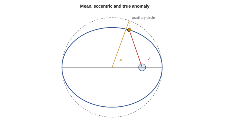
The mean anomaly grows uniformly with time from the moment of perigee passage:

where \(n\) is the mean motion in radians per second. Kepler's equation links mean and eccentric anomaly:

and the eccentric anomaly links to the true anomaly through

The radius follows directly from the eccentric anomaly as \(r = a(1 - e\cos E)\). These three equations together answer both directions of the timing problem.

Time of flight: the easy direction

If the position is known and the time is wanted, the calculation runs straight through. Given \(\nu\), find \(E\) from the half-angle relation, then \(M\) from Kepler's equation, then \(t = M/n\). No iteration is needed. This is the calculation Lakeshore needs: how long after perigee passage, which happens close to engine cut-off, does their satellite reach apogee, where the circularization burn is made?

For their geostationary transfer orbit, 250 km by 35,786 km, the semi-major axis is 24,396 km and the eccentricity 0.7283. The period is 10.53 hours, so apogee comes after half a period, 5.27 hours. The more useful number is the time to reach a true anomaly of 90 degrees, a quarter of the way around in angle: only 0.43 hours, about 26 minutes. The satellite covers the first quarter of the angle in about 4 percent of the period because it moves so fast near perigee, then spends hours climbing slowly toward apogee. Mission planners use this asymmetry, for instance by placing ground stations so that they see the long, slow arc near apogee.

Position at a given time: the hard direction

The reverse problem is the one operations need: given a time, where is the satellite? Now \(M\) is known and \(E\) must be found from \(M = E - e\sin E\), an equation that cannot be solved for \(E\) in closed form. Kepler himself solved it by successive approximation. Modern software uses Newton's method, which converges very quickly for this equation. Starting from a guess \(E_0\), each step improves it by

A good starting value is \(E_0 = M\) for eccentricities below about 0.8 and \(E_0 = \pi\) for higher eccentricities, which avoids slow starts near perigee of very elongated orbits. With these starting values, Newton's method converges to machine precision in a handful of iterations for any elliptical orbit.

# Kepler's equation by Newton's method: where is a spacecraft at a given time, and how long to reach a given point?
import math
MU = 398600.4418; RE = 6378.137
def kepler_E(M, e, tol=1e-12):
    E = M if e < 0.8 else math.pi
    for k in range(50):
        dE = (E - e*math.sin(E) - M) / (1 - e*math.cos(E))
        E -= dE
        if abs(dE) < tol: return E, k + 1
    raise RuntimeError("no convergence")
def nu_from_E(E, e): return 2*math.atan2(math.sqrt(1+e)*math.sin(E/2), math.sqrt(1-e)*math.cos(E/2))
def tof(nu, e, n):
    E = 2*math.atan2(math.sqrt(1-e)*math.sin(nu/2), math.sqrt(1+e)*math.cos(nu/2))
    if E < 0: E += 2*math.pi
    return (E - e*math.sin(E)) / n
# A geostationary transfer orbit flown by a weather satellite: 250 km by 35,786 km
rp, ra = RE + 250, RE + 35786
a = (rp + ra)/2; e = (ra - rp)/(ra + rp); n = math.sqrt(MU/a**3)
print(f"GTO a = {a:.0f} km, e = {e:.4f}, period = {2*math.pi/n/3600:.3f} h")
for t_h in (0.5, 1.0, 2.0, 5.0):
    M = n * t_h * 3600
    E, it = kepler_E(M % (2*math.pi), e)
    nu = nu_from_E(E, e); r = a*(1 - e*math.cos(E))
    print(f"t = {t_h:3.1f} h: M = {math.degrees(M):7.2f} deg, E = {math.degrees(E):7.2f} deg ({it} iterations), "
          f"nu = {math.degrees(nu)%360:7.2f} deg, altitude = {r - RE:8.0f} km")
for nu_deg in (90, 180):
    print(f"time from perigee to nu = {nu_deg} deg: {tof(math.radians(nu_deg), e, n)/3600:.3f} h")

GTO a = 24396 km, e = 0.7283, period = 10.534 h
t = 0.5 h: M =   17.09 deg, E =   48.19 deg (6 iterations), nu =   96.88 deg, altitude =     6173 km
t = 1.0 h: M =   34.18 deg, E =   74.36 deg (6 iterations), nu =  124.81 deg, altitude =    13228 km
t = 2.0 h: M =   68.35 deg, E =  108.03 deg (6 iterations), nu =  147.88 deg, altitude =    23518 km
t = 5.0 h: M =  170.88 deg, E =  174.72 deg (4 iterations), nu =  177.90 deg, altitude =    35711 km
time from perigee to nu = 90 deg: 0.429 h
time from perigee to nu = 180 deg: 5.267 h

The output shows the uneven pace of an eccentric orbit. Half an hour after perigee the satellite is already 6200 km up and has swept nearly 97 degrees of true anomaly. After five hours it is just short of apogee, at 35,700 km, having taken the remaining 81 degrees slowly. Newton's method needed at most six iterations. Arjun includes the iteration count in the output on purpose: a routine that suddenly needs 30 iterations is a sign of a bad starting guess or an orbit that is not elliptical.

Orbit determination and the epoch

Every timing calculation starts from an epoch: the moment at which the orbit elements or the state vector are known. For Crocus-1 the epoch comes from the onboard GNSS receiver, which measures position to a few metres and velocity to a few centimetres per second. On the ground, the flight dynamics software fits an orbit to a day of these measurements by least squares, adjusting the six elements and a drag parameter until the predicted positions match the measured ones as closely as possible. The fitted orbit is then propagated forward to predict passes and imaging opportunities. Older satellites without GNSS rely on ranging from ground stations or on radar and optical tracking, and the two-line element sets distributed for most catalogued objects come from this kind of tracking.

The quality of a prediction falls with time from the epoch. Position errors grow fastest along the track, because a small error in the semi-major axis produces an error in the period and that error accumulates every revolution. If the semi-major axis is wrong by 10 metres at 550 km, the period is wrong by about 0.012 seconds; after 100 revolutions, about a week, the along-track error is roughly 9 km. Drag uncertainty adds a larger effect at low altitude, because the atmosphere's density changes with solar activity. This is why Arjun refreshes the orbit daily and why the imaging plan is never built more than a day or two ahead.

Series solutions and when to use them

For small eccentricities, Kepler's equation can be inverted as a power series in \(e\). To first order, \(E \approx M + e\sin M\), and the true anomaly is approximately \(\nu \approx M + 2e\sin M\). For Crocus-1, whose eccentricity is about 0.001, the first-order error is a few millionths of a radian, smaller than a metre along the orbit, so these expressions are perfectly adequate for quick planning. The difference \(2e\sin M\), called the equation of centre, is the same quantity astronomers used for centuries to correct the position of the Sun in the sky. For eccentric orbits such as the transfer orbit the series converges slowly or not at all, and Newton's method is the safe choice. Good software does not choose between them by hand: it uses a short series to produce the starting guess and Newton's method to finish.

Hyperbolic and near-parabolic cases

For a hyperbola the eccentric anomaly is replaced by a hyperbolic anomaly \(F\), and Kepler's equation becomes \(M_h = e\sinh F - F\), with \(M_h\) growing uniformly in time. Departure and arrival hyperbolas in Lesson 8 use this form. Near \(e = 1\) both the elliptical and hyperbolic forms become numerically delicate, because small errors in \(e\) produce large errors in time. Robust software uses universal variables, a single formulation that works for all conic sections and passes smoothly through the parabolic case. The division adopts a universal-variable routine for operations and keeps the classical form for teaching and quick checks.

Timing ground contacts

For Crocus-1 the timing problem is mostly about ground contacts. The satellite downloads images to a ground station near Winnipeg and to partner stations at high latitude, where polar orbits pass on almost every revolution. A contact begins when the satellite rises above the station's elevation mask, typically 5 to 10 degrees to stay clear of buildings and trees, and ends when it sets. On a nearly circular orbit the time between rising and setting follows from geometry alone, as Lesson 11 shows: about 10 minutes on an overhead pass at 550 km with a 5-degree mask. Predicting the start of each pass to within a second needs the full propagator with perturbations, and the operations team updates the orbit from GNSS data every day to keep predictions accurate.

Imaging needs the same timing. Dr. Benali's crop maps require images over particular fields; the camera must be switched on and pointed seconds before the satellite reaches the target. An error of one second in time is a 7.6 km error along the track, larger than a typical field. The imaging schedule is therefore computed from the latest orbit solution and uploaded with each daily command plan.

Lambert's problem

A related problem appears whenever the team plans a transfer between two known positions. Lambert's problem asks: given two position vectors and the time to fly between them, what orbit connects them? It has a unique answer for each choice of transfer direction and number of revolutions, and it is solved numerically with the same tools as Kepler's equation. Lambert solvers are the workhorse of interplanetary mission design, where porkchop plots of launch date against arrival date are built from thousands of Lambert solutions. They are also used in rendezvous planning, where a servicing vehicle must reach a target at a chosen time.