
AERO-420 · Lesson 2 of 12 · 26 min
Orbital elements
A propagator works with a state vector: three components of position and three of velocity at one instant. Six numbers are enough to fix an orbit in the two-body problem, but state vectors are hard to read. Nobody can look at \((-1660, 3138, 5941)\) km and \((-1.219, 6.484, -3.759)\) km/s and say whether the satellite is in a useful orbit. Mission designers therefore describe orbits with six classical orbital elements, each with a clear physical meaning. This lesson defines them, shows how to convert between elements and state vectors, and uses them to write the Crocus-1 orbit specification.
Arjun needs the conversion for a practical reason. Launch providers quote the separation orbit as elements, ground stations need state vectors to point their antennas, and the tracking data that comes back after launch arrives as either one or the other, often in the two-line element format used by the public catalogue of tracked objects. The team cannot afford a mistake in the conversion, so Arjun writes it once, tests it both ways, and uses that one routine everywhere.
The six classical elements
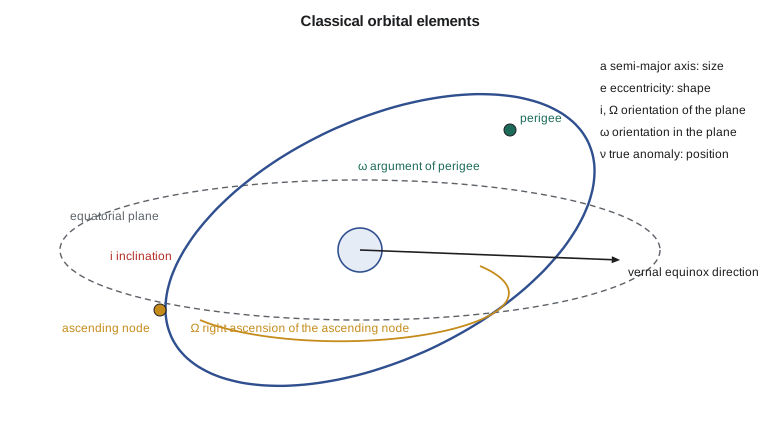
Two elements describe the size and shape of the orbit in its own plane. The semi-major axis \(a\) is half the longest diameter of the ellipse and fixes the energy and the period. The eccentricity \(e\) fixes the shape, from 0 for a circle toward 1 for a long, thin ellipse. Crocus-1's target orbit has \(a = 6928.1\) km and \(e = 0.0012\): nearly circular, with perigee and apogee about 17 km apart, a small eccentricity that comes naturally from Earth's uneven gravity, as Lesson 6 explains.
Three elements orient the orbit plane and the ellipse in space. The inclination \(i\) is the angle between the orbit plane and Earth's equator, measured from 0 to 180 degrees. An orbit with \(i < 90^\circ\) is prograde, moving eastward with Earth's rotation; above 90 degrees it is retrograde. Crocus-1 has \(i = 97.59^\circ\), slightly retrograde, which is what a sun-synchronous orbit at 550 km requires.
The orbit plane crosses the equator at two points called nodes. The ascending node is where the satellite crosses northward. The right ascension of the ascending node, \(\Omega\), is the angle in the equatorial plane from the vernal equinox direction to the ascending node. Together, \(i\) and \(\Omega\) fix the plane. Within the plane, the argument of perigee \(\omega\) is the angle from the ascending node to perigee, measured in the direction of motion. Finally, the true anomaly \(\nu\) gives the satellite's position along the orbit at a chosen time, the epoch.
| Element | Symbol | What it controls | Crocus-1 target |
|---|---|---|---|
| Semi-major axis | \(a\) | size, energy, period | 6928.1 km |
| Eccentricity | \(e\) | shape | 0.0012 |
| Inclination | \(i\) | tilt of the plane, latitudes covered | \(97.59^\circ\) |
| Right ascension of the ascending node | \(\Omega\) | plane orientation around the pole, local time of passes | set by launch time |
| Argument of perigee | \(\omega\) | where perigee lies in the plane | about \(90^\circ\) (frozen orbit) |
| True anomaly at epoch | \(\nu\) | where the satellite is at the epoch | set by separation time |
Elements and what users care about
Each element maps onto something a customer or operator feels. The inclination sets the highest latitude the ground track reaches: \(i\) for prograde orbits and \(180^\circ - i\) for retrograde ones. With \(i = 97.59^\circ\), Crocus-1 reaches 82.4 degrees north and south, so every part of Manitoba lies well inside its coverage. The semi-major axis sets the period and therefore how the ground track shifts westward from one orbit to the next, about \(360^\circ \times 95.6/1436 = 24.0^\circ\) of longitude per orbit at the equator.
The node \(\Omega\), measured against the stars, determines the local time at which the satellite crosses the equator. Dr. Benali wants crossings at 10:30 in the morning on the descending pass: late enough that the Sun is well above the horizon over the farms, early enough that afternoon convective clouds have not yet formed. Because Earth moves around the Sun, a fixed \(\Omega\) would let that local time drift by four minutes a day; Lesson 6 shows how Earth's oblateness is used to make \(\Omega\) turn at exactly the right rate.
The argument of perigee matters most for elliptical orbits, where it decides over which part of the Earth the satellite is high or low. For a nearly circular orbit like Crocus-1, the team chooses a frozen orbit: an eccentricity and argument of perigee, about 0.001 and 90 degrees, at which Earth's uneven gravity no longer makes them drift. The altitude over any given latitude then repeats from orbit to orbit, which keeps image resolution consistent.
Singular cases and alternative elements
The classical elements break down in two common cases. For a circular orbit, perigee is undefined, so \(\omega\) and \(\nu\) cannot be separated; designers use the argument of latitude \(u = \omega + \nu\), measured from the ascending node. For an equatorial orbit, the node is undefined, so \(\Omega\) and \(\omega\) merge into the longitude of perigee. Software that converts state vectors to elements must handle these cases, or it will divide by zero for exactly the orbits that missions use most. Many operational tools therefore use equinoctial elements, a set built from combinations of the classical ones that stays well behaved for circular and equatorial orbits.
Two-line element sets, the format in which the public catalogue of tracked objects is distributed, use mean elements fitted to tracking data with a particular simplified perturbation model. They are not the same as the osculating elements that Arjun's conversion produces from an instantaneous state vector. Using a two-line element set with any propagator other than the one it was fitted for can introduce errors of kilometres within a day. The team uses the published sets only for initial acquisition after launch, then switches to its own orbit determination from GNSS data.
From elements to a state vector
The conversion from elements to position and velocity is done in two steps. First, the position and velocity are written in the perifocal frame, whose \(x\)-axis points to perigee and whose \(z\)-axis is along the angular momentum:
where \(p = a(1 - e^{2})\) is the semi-latus rectum. Second, the vectors are rotated into the inertial frame by three successive rotations: by \(\omega\) about the perifocal \(z\)-axis, by \(i\) about the line of nodes, and by \(\Omega\) about Earth's polar axis. The product of the three rotations is a single \(3 \times 3\) matrix whose entries are sines and cosines of the three angles.
From a state vector to elements
The reverse conversion uses the invariants from Lesson 1. The angular momentum \(\mathbf{h} = \mathbf{r} \times \mathbf{v}\) gives the inclination from its \(z\)-component, \(\cos i = h_z/h\). The node vector \(\mathbf{N} = \hat{\mathbf{k}} \times \mathbf{h}\) points to the ascending node and gives \(\Omega\). The eccentricity vector points to perigee and has length \(e\):
The argument of perigee is the angle between \(\mathbf{N}\) and \(\mathbf{e}\), and the true anomaly the angle between \(\mathbf{e}\) and \(\mathbf{r}\). Each angle comes from an inverse cosine, which only returns values from 0 to 180 degrees, so the quadrant must be fixed with a sign test: \(\Omega\) is in the second half if \(N_y < 0\), \(\omega\) if \(e_z < 0\), and \(\nu\) if the satellite is moving toward Earth, \(\mathbf{r}\cdot\mathbf{v} < 0\). Forgetting these tests is the most common bug in student code, and it puts the satellite on the wrong side of the Earth.
# Classical orbital elements from a state vector and back again (Curtis-style algorithms).
import math
MU = 398600.4418
def norm(x): return math.sqrt(sum(c*c for c in x))
def cross(a, b): return [a[1]*b[2]-a[2]*b[1], a[2]*b[0]-a[0]*b[2], a[0]*b[1]-a[1]*b[0]]
def dot(a, b): return sum(x*y for x, y in zip(a, b))
def rv2coe(r, v):
    h = cross(r, v); hn = norm(h)
    i = math.degrees(math.acos(h[2]/hn))
    N = cross([0, 0, 1], h); Nn = norm(N)
    raan = math.degrees(math.acos(N[0]/Nn)); raan = raan if N[1] >= 0 else 360 - raan
    rn, vr = norm(r), dot(r, v)/norm(r)
    e_vec = [((norm(v)**2 - MU/rn)*r[k] - rn*vr*v[k])/MU for k in range(3)]; e = norm(e_vec)
    w = math.degrees(math.acos(dot(N, e_vec)/(Nn*e))); w = w if e_vec[2] >= 0 else 360 - w
    nu = math.degrees(math.acos(dot(e_vec, r)/(e*rn))); nu = nu if vr >= 0 else 360 - nu
    a = hn**2/MU/(1 - e*e)
    return a, e, i, raan, w, nu
def coe2rv(a, e, i, raan, w, nu):
    i, raan, w, nu = map(math.radians, (i, raan, w, nu))
    p = a*(1 - e*e); r_pf = p/(1 + e*math.cos(nu))
    rp = [r_pf*math.cos(nu), r_pf*math.sin(nu), 0]
    vp = [-math.sqrt(MU/p)*math.sin(nu), math.sqrt(MU/p)*(e + math.cos(nu)), 0]
    cO, sO, ci, si, cw, sw = math.cos(raan), math.sin(raan), math.cos(i), math.sin(i), math.cos(w), math.sin(w)
    row1 = [cO*cw - sO*sw*ci, -cO*sw - sO*cw*ci, sO*si]
    row2 = [sO*cw + cO*sw*ci, -sO*sw + cO*cw*ci, -cO*si]
    row3 = [sw*si, cw*si, ci]
    Q = [row1, row2, row3]
    mul = lambda M, x: [sum(M[r][c]*x[c] for c in range(3)) for r in range(3)]
    return mul(Q, rp), mul(Q, vp)
# Crocus-1 target orbit: nearly circular sun-synchronous, 550 km
elems = (6928.137, 0.0012, 97.59, 285.0, 90.0, 30.0)
r, v = coe2rv(*elems)
print("state vector r (km):", [round(x, 3) for x in r])
print("state vector v (km/s):", [round(x, 5) for x in v])
back = rv2coe(r, v)
labels = ("a km", "e", "i deg", "RAAN deg", "arg perigee deg", "true anomaly deg")
for lab, x0, x1 in zip(labels, elems, back):
print(f"{lab:17s} in {x0:10.4f} out {x1:10.4f}")state vector r (km): [-1660.328, 3137.656, 5941.192] state vector v (km/s): [-1.21864, 6.4835, -3.75932] a km in 6928.1370 out 6928.1370 e in 0.0012 out 0.0012 i deg in 97.5900 out 97.5900 RAAN deg in 285.0000 out 285.0000 arg perigee deg in 90.0000 out 90.0000 true anomaly deg in 30.0000 out 30.0000
The round trip returns all six elements to four decimal places, which confirms both routines and their quadrant tests. Arjun adds further test cases at the singular points, an exactly circular orbit and an equatorial one, and checks that the code reports the argument of latitude or longitude of perigee instead of failing.
Writing the orbit specification
The orbit specification is the document that the launch provider, the operations team and the regulators all work from. For Crocus-1 it states the target elements with tolerances: semi-major axis within 10 km, inclination within 0.1 degree, and the local time of the descending node at 10:30 within 15 minutes. It also states which reference frame and epoch the elements are given in, because an inclination quoted in a frame tied to a different date can differ by small but real amounts. The tolerances are not arbitrary: Lesson 4 shows how much propellant it costs to fix a semi-major axis error, and Lesson 5 shows why an inclination error is far more expensive.
Worked problem
Highest latitude reached
What is the highest latitude Crocus-1 reaches, and does its ground track pass over Winnipeg at latitude 49.9 degrees north?
Show solution
- For a retrograde orbit the highest latitude is \(180^\circ - i = 180^\circ - 97.59^\circ = 82.41^\circ\).
- Winnipeg at 49.9 degrees north is below 82.41 degrees, so ground tracks cross its latitude twice an orbit.
Answer: 82.4 degrees; every point between 82.4 degrees south and north is overflown.
Worked problem
Ground track shift
How far west does the ground track move between consecutive equator crossings?
Show solution
- Earth turns \(360^\circ\) in one sidereal day of 1436 minutes.
- During one 95.6-minute orbit it turns \(360 \times 95.6/1436 = 24.0^\circ\).
Answer: About 24 degrees of longitude, roughly 2670 km at the equator; at 49.9 degrees north the spacing shrinks with the cosine of latitude.
Worked problem
Reading an angular momentum vector
A state vector gives \(\mathbf{h} = (6930, -51\,600, -6990)\ \mathrm{km^2/s}\). Find the inclination.
Show solution
- \(h = \sqrt{6930^{2} + 51600^{2} + 6990^{2}} = 52\,530\ \mathrm{km^2/s}\).
- \(\cos i = -6990/52530 = -0.1331\), so \(i = 97.65^\circ\).
Answer: About 97.6 degrees: a retrograde, nearly polar orbit.
Common mistakes
MistakeUsing an inverse cosine without checking the quadrant.
InsteadApply the sign tests on \(N_y\), \(e_z\) and \(\mathbf{r}\cdot\mathbf{v}\).
MistakeComputing \(\omega\) and \(\nu\) separately for a circular orbit.
InsteadUse the argument of latitude \(u = \omega + \nu\).
MistakePropagating two-line element sets with a general integrator.
InsteadUse them with the simplified model they were fitted for, or only for initial acquisition.
MistakeQuoting elements without a frame and epoch.
InsteadState the reference frame and time; small differences matter for tolerances.
MistakeAssuming inclination above 90 degrees is an error.
InsteadIt means retrograde motion; sun-synchronous orbits need it.
Summary and key terms
- Six classical orbital elements describe an orbit in terms people can read.
- Semi-major axis and eccentricity set size and shape; inclination and the right ascension of the ascending node set the plane; argument of perigee sets the ellipse within the plane; true anomaly gives position at an epoch.
- Conversions to and from state vectors use rotation matrices one way and the angular momentum, node and eccentricity vectors the other way, with careful quadrant checks.
- Circular and equatorial orbits need alternative elements.
- The Crocus-1 specification sets elements with tolerances in a stated frame.
- Orbital elements
- Six numbers that describe the size, shape, orientation and phase of an orbit.
- Inclination
- The angle between the orbit plane and the equator.
- Ascending node
- The point where the orbit crosses the equator going north.
- Argument of perigee
- The angle from the ascending node to perigee.
- Argument of latitude
- The angle from the ascending node to the satellite; used for circular orbits.
- Perifocal frame
- A frame with its x-axis toward perigee and z-axis along the angular momentum.
- Frozen orbit
- A choice of eccentricity and argument of perigee that does not drift under zonal gravity.
- Two-line element set
- Mean elements fitted to tracking data for use with one simplified model.
Practice problems
Work each problem on paper first, then reveal the answer to check.
What does \(\cos i = h_z/h\) give for an equatorial prograde orbit?
Show answer
\(i = 0\).
Which element is undefined for a circular orbit?
Show answer
The argument of perigee, and with it the true anomaly.
Why does Dr. Benali care about \(\Omega\)?
Show answer
It sets the local time of the passes, which controls Sun angle and cloud.
How many numbers define a two-body orbit?
Show answer
Six.
What sign test fixes the quadrant of the true anomaly?
Show answer
If \(\mathbf{r}\cdot\mathbf{v} < 0\), the satellite approaches perigee and \(\nu\) is between 180 and 360 degrees.
What is the highest latitude of an orbit with \(i = 51.6^\circ\)?
Show answer
51.6 degrees.
Lesson quiz · 5 questions
Score 60% or more to complete this lesson.
Create a free account to save your progress, take quizzes and earn a certificate.