
ACCT-341 · Lesson 7 of 12 · 28 min
Descriptive and diagnostic analytics: distributions, ratios and variances
With clean, reconciled data and the means to query it, the analyst can start answering questions. This lesson covers the two kinds of analytics accountants use most: describing what happened and diagnosing why. It begins with describing distributions, because accounting data have a shape that trips up people used to textbook statistics. It then covers comparisons, ratios and trends, and finishes with two diagnostic techniques that close the Cedarbrook margin story: drilling down by segment and decomposing a change in gross profit into price, cost, volume and mix effects. You should already know basic descriptive statistics from STAT-141; the focus here is on applying them to accounting data.
Describing a distribution
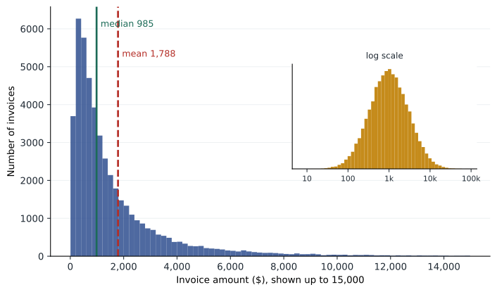
Most accounting populations, such as invoice amounts, payments, expense claims and inventory values, are strongly right-skewed. There are many small items and a few very large ones. That shape has practical consequences. The mean is pulled up by the large items and is a poor guide to a typical transaction; the median is better. The standard deviation is inflated by the tail and is a poor guide to normal variation; percentiles and the interquartile range are better. And a small share of items usually holds a large share of the value, which is why auditors stratify populations and test large items separately.
# Describing a skewed distribution: 2025 invoice amounts (simulated)
import numpy as np
import pandas as pd
rng = np.random.default_rng(7)
amounts = pd.Series(np.round(rng.lognormal(mean=6.9, sigma=1.1, size=48_000), 2))
s = amounts.describe(percentiles=[0.25, 0.5, 0.75, 0.99])
print(s.round(2).to_string())
print("skewness:", round(amounts.skew(), 2))
top = amounts.sort_values(ascending=False)
share = top.head(len(top) // 10).sum() / top.sum()
print(f"largest 10% of invoices hold {share:.0%} of the dollar value")
q1, q3 = amounts.quantile([0.25, 0.75])
fence = q3 + 3 * (q3 - q1)
print(f"invoices above the outer fence ({fence:,.0f}):", (amounts > fence).sum())count 48000.00 mean 1788.47 std 2635.72 min 7.01 25% 472.78 50% 985.34 75% 2076.13 99% 12342.29 max 86488.52 skewness: 6.45 largest 10% of invoices hold 42% of the dollar value invoices above the outer fence (6,886): 1793
The simulated invoices for 2025 total about 86 million. The mean invoice is about 1,790 dollars, but the median is only about 985: half of all invoices are smaller than that. The skewness of 6.45 confirms a long right tail, and the largest invoice is over 86,000. The largest tenth of invoices holds 42 per cent of the dollar value. An audit approach that tested a random sample of invoices with equal probability would spend most of its effort on small items; a stratified approach that tested all invoices over a threshold plus a sample of the rest would cover far more value with the same effort.
The last line shows a limitation of a common outlier rule. Tukey's fences flag values more than 1.5 or, for extreme outliers, 3 interquartile ranges above the third quartile. On skewed data, even the outer fence flags 1,793 invoices, nearly 4 per cent of the population, because the tail is a normal feature of the data, not a sign of error. Rules designed for symmetric data need adapting: analysts often apply them to the logarithm of the amounts, which makes skewed accounting data roughly symmetric, or use business-based thresholds such as amounts above a customer's credit limit.
| Measure | What it shows | Caution with accounting data |
|---|---|---|
| Mean | Arithmetic average | Pulled up by large items; not a typical value |
| Median | The middle value | Robust to large items; preferred for typical size |
| Standard deviation | Spread around the mean | Inflated by the tail |
| Percentiles and IQR | Values below which a share of items fall | Robust; good for thresholds |
| Skewness | Asymmetry of the distribution | Usually strongly positive |
| Concentration (top-share) | Share of value in the largest items | Guides stratification and coverage |
Comparisons give numbers meaning
A number on its own says little. Revenue of 86 million is good or bad only in comparison with something: last year, the budget, a forecast, a competitor, or the activity that should have generated it. Analytical work in accounting is largely the art of choosing the right comparison.
| Comparison | Example | Strength | Weakness |
|---|---|---|---|
| Prior period | Sales this quarter versus the same quarter last year | Easy; controls for seasonality if same period | Assumes last year was normal |
| Budget or forecast | Actual versus budget by branch | Reflects expectations and plans | Budgets can be biased or stale |
| Other units | One branch versus the others | Same company, same systems | Units may differ in mix or market |
| Industry or peers | Gross margin versus published peer data | External benchmark | Definitions and mix differ |
| Non-financial drivers | Freight cost per shipment; payroll per employee | Links money to activity; hard to manipulate | Driver data must be reliable |
Comparisons with non-financial data are especially valuable because they relate accounting numbers to physical reality. If Cedarbrook's freight expense rose 18 per cent but the number of shipments and the average distance did not change, something other than activity explains the increase. Auditors use the same idea in substantive analytical procedures, building an expectation from independent data and comparing it with the recorded amount, as lesson 11 describes.
Ratios and trends
Ratios scale one number by another so that units of different sizes, or periods with different activity, can be compared. You will know the standard financial ratios from earlier courses. For operational analysis, a few ratios do most of the work in a distribution business like Cedarbrook.
| Ratio | Formula | What a change may signal |
|---|---|---|
| Gross margin | (Revenue − cost of sales) ÷ revenue | Pricing, mix, purchase costs, costing errors |
| Days sales outstanding (DSO) | Receivables ÷ revenue × days in period | Collection problems, extended terms, fictitious sales |
| Days payables outstanding (DPO) | Payables ÷ cost of sales × days | Cash management, supplier stress, unrecorded liabilities |
| Inventory turnover | Cost of sales ÷ average inventory | Slow-moving or obsolete stock, overstatement |
| Operating expense ratio | Operating expenses ÷ revenue | Cost control, misclassification |
| Revenue per employee | Revenue ÷ average staff | Productivity; implausible revenue |
Trend analysis looks at how a measure moves over many periods, which reveals patterns a single comparison misses: steady erosion, seasonality, a step change at a particular date. Horizontal analysis expresses each line as a change from a base period; vertical analysis expresses each line as a percentage of a total, such as revenue, so that the structure of the income statement can be compared across periods of different size. Both are simple and powerful, and both are easy to do with the grouping and pivoting techniques from lesson 4.
Drilling down
Diagnosis usually proceeds by drilling down: breaking a total into components along one dimension, finding where the change is concentrated, and then breaking that component down along another dimension. In lesson 1, Maya found that Cedarbrook's margin decline was concentrated in the West region. Now she drills into West by customer.
# Drilling into the West region: margin by customer, 2024 vs 2025
import pandas as pd
west = pd.DataFrame({
    "customer": ["Ridge Homes", "Lakeview Mechanical", "Aspen Builders",
                 "Other customers"] * 2,
    "year":     [2024] * 4 + [2025] * 4,
    "revenue":  [0.0, 2.9, 1.6, 6.8, 3.4, 3.0, 1.5, 6.0],   # $ millions
    "cogs":     [0.0, 2.2, 1.2, 5.2, 3.1, 2.3, 1.1, 5.0],
})
g = west.groupby(["customer", "year"])[["revenue", "cogs"]].sum().unstack()
gp = (g["revenue"] - g["cogs"]).round(2)
out = pd.DataFrame({"rev_2024": g["revenue"][2024], "rev_2025": g["revenue"][2025],
                    "gp_2024": gp[2024], "gp_2025": gp[2025]})
out["margin_2025"] = (100 * out["gp_2025"] / out["rev_2025"]).round(1)
out["gp_change"] = out["gp_2025"] - out["gp_2024"]
print(out.sort_values("gp_change").round(2).to_string())
print("total gross profit change:", round(out["gp_change"].sum(), 2))rev_2024 rev_2025 gp_2024 gp_2025 margin_2025 gp_change customer Other customers 6.8 6.0 1.6 1.0 16.7 -0.6 Aspen Builders 1.6 1.5 0.4 0.4 26.7 0.0 Lakeview Mechanical 2.9 3.0 0.7 0.7 23.3 0.0 Ridge Homes 0.0 3.4 0.0 0.3 8.8 0.3 total gross profit change: -0.3
The result is more interesting than a single bad contract. Ridge Homes, a homebuilder that was not a customer in 2024, bought 3.4 million in 2025 at a margin of only 8.8 per cent. On its own that is a thin but positive contribution: it added 0.3 million of gross profit. The bigger problem is elsewhere. West's other customers, taken together, bought less and earned a margin of 16.7 per cent in 2025, down from about 23.5 per cent, losing 0.6 million of gross profit. The large customers Lakeview and Aspen held steady. Maya's hypothesis now is that something done to win or serve Ridge Homes spread to the rest of the branch.
Price, cost, volume and mix
A standard way to explain a change in gross profit is to decompose it into effects. The volume effect is the change from selling more or fewer units at the old average margin. The mix effect is the change from selling a different combination of products, some more profitable than others. The price effect is the change from charging different prices on the units actually sold, and the cost effect is the change from paying different costs. There are several ways to define these effects, and they give slightly different splits, so the method should be stated. The one used here is common and has the useful property that the effects add up exactly to the total change.
Here Q is total units, s the share of units in each category, m the margin per unit, p the price and c the unit cost, with subscripts 0 and 1 for the two years and the bar marking the old weighted average margin. Maya applies the decomposition to West's three product categories, using unit data from the item master and sales history.
# Price, cost, mix and volume effects on West gross profit, 2024 to 2025
import pandas as pd
d = pd.DataFrame({
    "category": ["Pipe and fittings", "Fixtures", "HVAC equipment"],
    "qty0":   [52.0, 18.0, 6.0],    "qty1":   [55.0, 31.0, 6.5],   # 000 units
    "price0": [95.0, 220.0, 410.0], "price1": [94.0, 196.0, 412.0],
    "cost0":  [70.0, 172.0, 316.0], "cost1":  [72.0, 176.0, 318.0],
})
d["gm0"] = d["price0"] - d["cost0"]                 # margin per unit
d["gm1"] = d["price1"] - d["cost1"]
Q0, Q1 = d["qty0"].sum(), d["qty1"].sum()
avg_gm0 = (d["qty0"] * d["gm0"]).sum() / Q0
volume = (Q1 - Q0) * avg_gm0
mix = (Q1 * (d["qty1"] / Q1 - d["qty0"] / Q0) * d["gm0"]).sum()
price = (d["qty1"] * (d["price1"] - d["price0"])).sum()
cost = -(d["qty1"] * (d["cost1"] - d["cost0"])).sum()
gp0 = (d["qty0"] * d["gm0"]).sum()
gp1 = (d["qty1"] * d["gm1"]).sum()
for name, v in [("2024 gross profit", gp0), ("volume effect", volume),
                ("mix effect", mix), ("price effect", price),
                ("cost effect", cost), ("2025 gross profit", gp1)]:
    print(f"{name:<20}{v / 1000:>8.2f}")        # $ millions
print("check:", round(gp0 + volume + mix + price + cost - gp1, 6))2024 gross profit 2.73 volume effect 0.59 mix effect 0.15 price effect -0.79 cost effect -0.25 2025 gross profit 2.44 check: 0.0
West's gross profit fell from 2.73 million to 2.44 million. Selling more units added 0.59 million, and a shift toward fixtures, which carry a higher margin per unit than the average, added 0.15 million. Those gains were more than wiped out by lower prices, which cost 0.79 million, and higher purchase costs, which cost 0.25 million. Almost all of the price effect comes from fixtures, where the average price fell from 220 to 196 dollars, about 11 per cent. The check line confirms that the four effects reconcile exactly to the change in gross profit.
Putting the two analyses together, Maya has a clear diagnosis to test. West cut fixture prices sharply to win the Ridge Homes contract, and the lower prices appear to have spread to other West customers, perhaps because the branch updated its price list rather than setting a contract price for Ridge alone. She can now confirm this with evidence: the price list change history in the ERP, the Ridge Homes contract terms, and conversations with the West branch manager. The recommendation to the board will be specific: restore the standard fixture price list for customers other than Ridge, review the Ridge contract at renewal, and add a monthly margin-by-customer report to catch similar problems sooner.
Worked problem
Interpreting the decomposition
If West had kept fixture prices at 220 dollars while selling the same units, roughly how much higher would its 2025 gross profit have been?
Show solution
- The fixture price fell by 24 dollars per unit (220 − 196).
- West sold 31 thousand fixture units in 2025.
- 31,000 × 24 = 744,000 dollars.
- Gross profit would have been about 2.44 + 0.74 = 3.18 million, above 2024, assuming volumes did not depend on the price cut.
Answer: About 0.74 million higher, though in reality some of the extra volume, including the Ridge contract, may have depended on the lower price.
Cautions in diagnosis
Diagnostic analytics finds associations, and associations are not causes. Two measures can move together because one drives the other, because both are driven by a third factor, or by coincidence. Freight costs and sales both rise in the summer construction season; neither causes the other. Good diagnosis looks for a mechanism, a business reason why one thing would cause another, and then seeks evidence of the mechanism, as Maya did by planning to examine the price list history.
Aggregation can also mislead. Simpson's paradox is the name for a pattern that holds in every subgroup but reverses when the groups are combined, because the groups differ in size or mix. A company can see margins rise in every product category and still see overall margin fall, if sales shift toward lower-margin categories. That is one reason the mix effect exists as a separate component, and one reason analysts drill down rather than relying only on totals.
Finally, be wary of explanations that arrive too easily. Once a plausible story appears, there is a temptation to stop looking. Professional skepticism means checking whether the story explains the whole change, which the decomposition's check line helps with, and whether other evidence contradicts it.
Common mistakes
MistakeUsing the mean to describe a typical invoice.
InsteadUse the median and percentiles for skewed data; report the mean for totals.
MistakeApplying symmetric outlier rules to skewed data.
InsteadUse logs, business thresholds or stratification instead.
MistakeComparing only with last year.
InsteadUse several comparison bases, including budgets, other units and non-financial drivers.
MistakeExplaining a margin change with one cause when several are at work.
InsteadDecompose the change into volume, mix, price and cost effects that reconcile to the total.
MistakeTreating correlation as proof of cause.
InsteadIdentify a business mechanism and find evidence for it.
Summary and key terms
- Accounting populations are usually right-skewed; prefer the median, percentiles and concentration measures.
- A small share of large items often holds a large share of value, which supports stratification.
- Numbers gain meaning through comparison with prior periods, budgets, other units, peers and non-financial drivers.
- Gross margin, DSO, DPO, inventory turnover and expense ratios are key operational measures for a distributor.
- Drill down one dimension at a time to locate where a change is concentrated.
- Price, cost, volume and mix effects decompose a gross profit change and should reconcile exactly.
- At Cedarbrook, West's fixture price cuts cost 0.79 million and spread beyond the new Ridge Homes contract.
- Associations are not causes; look for mechanisms and beware Simpson's paradox.
- Median
- The middle value of a sorted set of numbers.
- Skewness
- A measure of the asymmetry of a distribution.
- Interquartile range (IQR)
- The difference between the 75th and 25th percentiles.
- Stratification
- Dividing a population into groups, such as by size, to analyse or test them separately.
- Horizontal analysis
- Comparing each line item with the same item in a base period.
- Vertical analysis
- Expressing each line item as a percentage of a total.
- Days sales outstanding
- Receivables divided by revenue, times the days in the period.
- Drill-down
- Breaking a total into components to find where a change is concentrated.
- Mix effect
- The part of a change caused by a different combination of products or customers.
- Simpson's paradox
- A pattern present in every subgroup that reverses when the groups are combined.
Practice problems
Work each problem on paper first, then reveal the answer to check.
Why is the median a better measure of a typical invoice than the mean?
Show answer
Large invoices pull the mean up; the median is not affected by them.
In the descriptive program, what share of dollar value is in the largest 10 per cent of invoices?
Show answer
42 per cent.
Change the outer fence in the program to use the logarithm of amounts. Why would this help?
Show answer
Log amounts are roughly symmetric, so the fence flags genuinely unusual values instead of the normal tail.
Receivables are 9.4 million and annual revenue 86 million. What is DSO on a 365-day basis?
Show answer
About 39.9 days.
In the customer program, how much gross profit did West's other customers lose?
Show answer
0.6 million.
What was the fixture price effect in the decomposition, approximately?
Show answer
About −0.74 million of the −0.79 million total price effect.
Change the 2025 fixture price in the decomposition program to 220. What happens to the price effect?
Show answer
It becomes about −0.04 million, from the small pipe and HVAC price changes.
Why must decomposition effects reconcile to the total change?
Show answer
Otherwise part of the change is unexplained, and the analysis may be wrong or incomplete.
Give an example of a non-financial driver for payroll expense.
Show answer
Average headcount or hours worked.
What is Simpson's paradox?
Show answer
A pattern in every subgroup that reverses when the groups are combined, due to differences in group size or mix.
Lesson quiz · 5 questions
Score 60% or more to complete this lesson.
Create a free account to save your progress, take quizzes and earn a certificate.