
ACCT-222 · Lesson 9 of 12 · 25 min
Standard costing II: overhead variances, capacity and journal entries
Direct materials and direct labour are traced to products, so their standards come straight from bills of materials and routings. Manufacturing overhead is different: it is applied to products through a predetermined rate, and part of it is fixed. This lesson analyses overhead in a standard costing system: how variable and fixed overhead rates are set, how the total overhead variance splits into spending, efficiency, budget and production-volume variances, what the production-volume variance does and does not mean, how the choice of capacity level affects reported costs, and how a standard cost system records all of this in the ledger and disposes of variances at year-end.
Setting overhead standards
Halden applies machining-department overhead to products using machine hours, the activity that best explains most of the department's overhead. The budget for the year separates variable overhead (power, lubricants, tooling wear, maintenance supplies) from fixed overhead (supervision, depreciation, insurance, the maintenance crew). Variable overhead is budgeted at $10 per machine hour. Fixed overhead is budgeted at $400,000 for the year. Together they make up the $600,000 machining pool used in the ABC system of lesson 4. To apply fixed overhead to products, Halden needs a denominator level of activity, the quantity of the allocation base used to compute the fixed overhead rate. Halden uses normal capacity of 20,000 machine hours, the average level of use expected over the next few years, giving a fixed overhead rate of $400,000 ÷ 20,000 = $20 per machine hour. The combined rate of $30 per machine hour matches the machining activity rate in lesson 4.
Each S-100 pump is allowed 0.5 machine hours in machining, so its standard machining overhead is 0.5 × ($10 + $20) = $15.00. Overhead is applied to production on the basis of the standard machine hours allowed for the actual output, not the actual hours used; this is what distinguishes standard costing from the normal costing of ACCT-102.
| Item | Budget | Actual |
|---|---|---|
| Variable overhead rate | $10 per machine hour | |
| Fixed overhead | $400,000 | $412,000 |
| Denominator level (normal capacity) | 20,000 machine hours | |
| Fixed overhead rate | $20 per machine hour | |
| Actual machine hours used | 19,000 | |
| Standard machine hours allowed for actual output | 18,500 | |
| Actual variable overhead | $196,000 |
Variable overhead variances
Variable overhead has a spending variance and an efficiency variance, computed like the price and efficiency variances for direct inputs, with machine hours playing the role of quantity.
In the equations AVOH is actual variable overhead, SR the standard variable overhead rate per machine hour, AH actual machine hours and SH standard machine hours allowed for actual output. The spending variance is $196,000 − $10 × 19,000 = $6,000 unfavourable: Halden spent more per machine hour actually used than the $10 standard, perhaps because power prices rose or tooling wore faster. The efficiency variance is $10 × (19,000 − 18,500) = $5,000 unfavourable: the department used 500 more machine hours than standard for its output, and variable overhead rises with machine hours.
The efficiency variance for variable overhead says nothing about how efficiently overhead items themselves were used. It measures the overhead consequence of using the allocation base inefficiently. If machine hours are high because of extra set-ups or a slow machine, the cause lies there, and the investigation should look at the machining process, not the overhead accounts.
Fixed overhead variances
Fixed overhead does not vary with activity in the short run, so there is no efficiency variance for it. Instead there are two variances. The budget (spending) variance compares actual fixed overhead with the budget. The production-volume variance compares the budgeted fixed overhead with the fixed overhead applied to production at the standard rate.
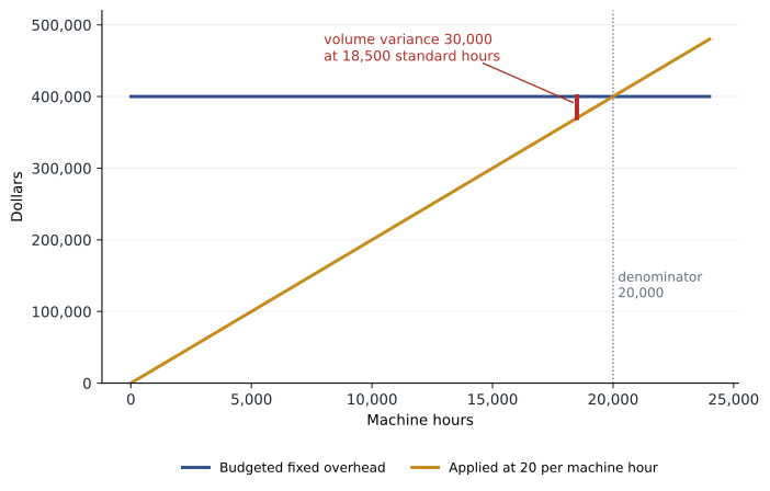
The budget variance is $412,000 − $400,000 = $12,000 unfavourable: Halden spent more on fixed overhead than budgeted, in this case because a supervisor's position was filled at a higher salary and insurance premiums rose. The production-volume variance is $400,000 − $20 × 18,500 = $400,000 − $370,000 = $30,000 unfavourable. Halden applied only $370,000 of fixed overhead to products because the output it produced was allowed 18,500 machine hours, below the 20,000-hour denominator.
# Four-way, three-way and two-way analysis of overhead (illustrative)
SR, FR = 10, 20                 # variable and fixed rates per machine hour
BFOH, denominator = 400_000, 20_000
AH, SH = 19_000, 18_500
AVOH, AFOH = 196_000, 412_000

voh_spending = AVOH - SR * AH
voh_efficiency = SR * (AH - SH)
foh_budget = AFOH - BFOH
volume = BFOH - FR * SH
applied = (SR + FR) * SH
actual = AVOH + AFOH

print("Four-way analysis (+ = U, - = F)")
for name, v in [("Variable OH spending", voh_spending), ("Variable OH efficiency", voh_efficiency),
                ("Fixed OH budget", foh_budget), ("Production-volume", volume)]:
    print(f"  {name:<24}{v:>+10,}")
print(f"Total under-applied overhead {actual - applied:+,} "
      f"(actual {actual:,} - applied {applied:,})")
print("Three-way: spending", f"{voh_spending + foh_budget:+,}", " efficiency",
      f"{voh_efficiency:+,}", " volume", f"{volume:+,}")
print("Two-way:   flexible-budget", f"{voh_spending + voh_efficiency + foh_budget:+,}",
" volume", f"{volume:+,}")Four-way analysis (+ = U, - = F) Variable OH spending +6,000 Variable OH efficiency +5,000 Fixed OH budget +12,000 Production-volume +30,000 Total under-applied overhead +53,000 (actual 608,000 - applied 555,000) Three-way: spending +18,000 efficiency +5,000 volume +30,000 Two-way: flexible-budget +23,000 volume +30,000
The four variances add to $53,000 unfavourable, which is exactly the overhead under-applied for the year: actual overhead of $608,000 less applied overhead of $30 × 18,500 = $555,000. Some companies present a three-way analysis, combining the two spending-type variances into one spending variance of $18,000, or a two-way analysis, combining everything except the production-volume variance into a flexible-budget variance of $23,000. The four-way analysis gives the most information and is used here.
What the production-volume variance means
The production-volume variance is the most misunderstood variance in standard costing. It arises only because fixed costs are converted into a per-unit rate for product costing. Halden's fixed overhead was going to be about $400,000 regardless of output; treating it as $20 per machine hour is an accounting device that makes inventory include fixed overhead. When output is below the denominator level, less fixed overhead is applied than budgeted, and the gap is labelled unfavourable. When output is above the denominator, more is applied than budgeted, and the variance is labelled favourable.
The variance does not measure a cash cost or a spending inefficiency. Producing more pumps would not reduce fixed overhead; it would simply spread it over more units. Its economic meaning, if any, is that capacity went unused: Halden supplied machining capacity for 20,000 hours of standard output and used only 18,500. Whether that unused capacity is a problem depends on why output was low. If demand was weak, the real cost is the lost contribution margin on sales that did not happen, which the production-volume variance does not measure. If output was low because of breakdowns while demand was strong, the cost is again lost contribution, and the efficiency variances and the sales department's records are better guides than the production-volume variance.
Managers should be wary of chasing a favourable production-volume variance by producing more than they can sell. Under absorption costing, overproduction moves fixed overhead into inventory, reduces the unfavourable variance and raises reported income in the current period, but it ties up cash in pumps that sit in the warehouse. ACCT-102 lesson 8 discussed this incentive; lesson 10 returns to it when comparing absorption, variable and throughput costing.
Choosing the denominator level
The fixed overhead rate depends on the denominator. There are four common choices, from largest to smallest:
- Theoretical capacity: the output possible if the plant ran at full efficiency all the time, with no breakdowns, set-ups or holidays. It is a benchmark rather than an achievable level.
- Practical capacity: theoretical capacity less unavoidable interruptions such as scheduled maintenance, holidays and set-ups.
- Normal capacity utilization: the average level of capacity use expected to satisfy demand over a period of two or three years, including seasonal and cyclical swings.
- Master-budget capacity utilization: the level of capacity use expected for the coming year only.
Halden's machining department could run 25,000 machine hours a year in theory, about 22,000 in practice, an expected average of 20,000 over the next three years, and 19,000 in the budget for this year.
# Effect of the denominator level on the fixed overhead rate and S-100 cost (illustrative)
BFOH = 400_000
mh_per_pump = 0.5
levels = {"Theoretical": 25_000, "Practical": 22_000,
          "Normal": 20_000, "Master budget": 19_000}
SH = 18_500
for name, hours in levels.items():
    rate = BFOH / hours
    per_pump = rate * mh_per_pump
    volume_var = BFOH - rate * SH
    print(f"{name:<14} rate ${rate:6.2f}/MH   fixed OH per S-100 ${per_pump:5.2f}   "
f"production-volume variance {volume_var:+10,.0f}")Theoretical rate $ 16.00/MH fixed OH per S-100 $ 8.00 production-volume variance +104,000 Practical rate $ 18.18/MH fixed OH per S-100 $ 9.09 production-volume variance +63,636 Normal rate $ 20.00/MH fixed OH per S-100 $10.00 production-volume variance +30,000 Master budget rate $ 21.05/MH fixed OH per S-100 $10.53 production-volume variance +10,526
The higher the denominator, the lower the fixed overhead rate, the lower the reported product cost, and the larger the unfavourable production-volume variance, because more of the fixed cost is treated as the cost of unused capacity rather than as a cost of products. A practical-capacity denominator gives a product cost that reflects only the capacity products actually need, which many experts favour for pricing: it avoids the downward demand spiral, in which low demand raises the per-unit cost under a budget-based denominator, prompting a price increase that further reduces demand and raises the cost again. It also highlights the cost of unused capacity as a separate figure that management can act on.
For external reporting, IAS 2 and ASPE Section 3031 require fixed production overhead to be allocated on the basis of the normal capacity of the production facilities. The actual level of production may be used if it approximates normal capacity. When production is abnormally low, the unallocated overhead is recognized as an expense in the period, rather than increasing the cost of each unit in inventory; when production is abnormally high, the amount allocated per unit is reduced so that inventory is not measured above cost.
Journal entries in a standard cost system
In a standard cost system, work in process, finished goods and cost of goods sold are carried at standard cost, and every variance is recorded in its own account when it arises. Halden's entries for the October foundry materials and assembly labour from lesson 8 illustrate the pattern for direct inputs:
| Entry | Debit | Credit |
|---|---|---|
| Purchase of materials at standard (price variance at purchase) | Materials inventory $43,920 (19,800 kg at standard prices: 15,600 × $1.20 + 4,200 × $6.00) | Accounts payable $43,860; DM price variance $60 (favourable) |
| Materials used | Work in process $38,880 (standard quantity allowed at standard price); DM efficiency variance $5,040 (unfavourable) | Materials inventory $43,920 |
| Direct labour | Work in process $58,320 (1,800 standard hours at the standard mix); DL rate variance $210; DL efficiency variance $2,200 (both unfavourable) | Wages payable $60,730 |
For overhead, actual costs are debited to variable and fixed overhead control accounts as incurred. Overhead is applied to work in process at standard: for the year, $185,000 of variable overhead ($10 × 18,500) and $370,000 of fixed overhead ($20 × 18,500), credited to variable and fixed overhead allocated accounts. At year-end the control and allocated accounts are closed, and the differences are recorded in the four overhead variance accounts.
Disposing of variances at year-end
At year-end the variance accounts must be closed. If the variances are immaterial, the simplest treatment is to write them all off to cost of goods sold. Inventories then remain at standard cost, which is acceptable for financial reporting when standards are current and approximate actual cost. If the variances are material, they should be prorated across the accounts that contain the year's standard costs (work in process, finished goods and cost of goods sold) so that inventory approximates actual cost, as accounting standards require. Abnormal amounts, such as costs from an unusual breakdown, are expensed and not prorated, consistent with the treatment of abnormal spoilage in lesson 3.
# Prorating the $53,000 under-applied overhead at year-end (illustrative)
variance = 53_000
standard_ohcost_in = {   # standard overhead contained in each account at year-end
    "Work in process": 27_750,
    "Finished goods": 55_500,
    "Cost of goods sold": 471_750,
}
total = sum(standard_ohcost_in.values())
print(f"Standard overhead applied in the year: {total:,}")
for acct, amt in standard_ohcost_in.items():
    share = variance * amt / total
print(f" {acct:<19} {amt:>8,} ({amt / total:5.1%}) receives {share:>8,.0f}")Standard overhead applied in the year: 555,000 Work in process 27,750 ( 5.0%) receives 2,650 Finished goods 55,500 (10.0%) receives 5,300 Cost of goods sold 471,750 (85.0%) receives 45,050
Proration based on the overhead each account contains is the most accurate method; a simpler alternative prorates on the accounts' total ending balances. Here about 85 per cent of the under-applied overhead goes to cost of goods sold and the rest increases inventory. If Halden judged the production-volume variance to reflect abnormally low output rather than normal fluctuation, it would expense that portion instead of prorating it, because standards allow only normal-capacity fixed overhead in inventory.
Standard costs also matter for government contracts. Under the Canadian federal Contract Cost Principles (SACC 1031-2), costs must be determined using the contractor's generally accepted, consistently applied accounting practices, so a contractor that uses standard costs must be able to show that variances are allocated reasonably to the work that caused them.
Common mistakes
MistakeApplying overhead on actual machine hours in a standard cost system.
InsteadApply overhead on the standard hours allowed for actual output.
MistakeComputing an efficiency variance for fixed overhead.
InsteadFixed overhead has a budget variance and a production-volume variance only.
MistakeTreating the production-volume variance as a cash cost of low output.
InsteadIt reflects the conversion of fixed costs to a unit rate; the real cost of low volume is lost contribution margin.
MistakeProducing extra inventory to eliminate an unfavourable production-volume variance.
InsteadOverproduction ties up cash and only defers fixed costs in inventory.
MistakeWriting material variances off to cost of goods sold without considering proration.
InsteadProrate material variances among work in process, finished goods and cost of goods sold, and expense abnormal amounts.
Summary and key terms
- Overhead is applied in a standard cost system on the standard quantity of the allocation base allowed for actual output.
- Variable overhead has spending and efficiency variances; the efficiency variance reflects inefficient use of the allocation base.
- Fixed overhead has a budget variance and a production-volume variance.
- The four variances add to the total under- or over-applied overhead; three-way and two-way analyses combine them.
- The production-volume variance arises from unitizing fixed costs and is not a measure of spending efficiency.
- Higher denominators lower product costs and enlarge the production-volume variance; practical capacity highlights unused capacity, while standards require normal capacity for inventory.
- Standard cost systems record variances as they arise and close them at year-end, prorating material variances and expensing abnormal amounts.
- Denominator level
- The quantity of the allocation base used to compute the fixed overhead rate.
- Variable overhead spending variance
- Actual variable overhead minus the standard rate times actual base quantity.
- Variable overhead efficiency variance
- The standard rate times the difference between actual and standard base quantity.
- Fixed overhead budget variance
- Actual fixed overhead minus budgeted fixed overhead.
- Production-volume variance
- Budgeted fixed overhead minus fixed overhead applied at the standard rate to actual output.
- Practical capacity
- Theoretical capacity less unavoidable interruptions.
- Normal capacity utilization
- The average expected level of capacity use over a period of two or three years.
- Downward demand spiral
- Rising unit costs and prices as demand falls, caused by spreading fixed costs over fewer units.
- Proration
- Spreading a variance among work in process, finished goods and cost of goods sold.
- Four-way analysis
- Splitting the total overhead variance into variable spending, variable efficiency, fixed budget and production-volume variances.
Practice problems
Work each problem on paper first, then reveal the answer to check.
Variable overhead rate $6 per labour hour; actual variable overhead $64,000; actual hours 10,200; standard hours 10,000. Compute the spending and efficiency variances.
Show answer
Spending 64,000 − 61,200 = $2,800 U; efficiency 6 × 200 = $1,200 U.
Budgeted fixed overhead $300,000; denominator 12,000 hours; standard hours allowed 12,600; actual fixed overhead $295,000. Compute the budget and production-volume variances.
Show answer
Rate $25; budget $5,000 F; applied $315,000; volume $15,000 F.
Why is the production-volume variance in the previous question favourable?
Show answer
Output exceeded the denominator, so more fixed overhead was applied than budgeted.
Compute Halden's fixed overhead rate if the denominator were practical capacity of 22,000 MH.
Show answer
$400,000 ÷ 22,000 ≈ $18.18 per MH.
With that rate, what is the production-volume variance at 18,500 standard hours?
Show answer
$400,000 − $336,364 ≈ $63,636 U.
Explain the downward demand spiral.
Show answer
As demand falls, a budget-based denominator raises the unit fixed cost; higher prices reduce demand further.
Halden's variances total $53,000 unfavourable. Which accounts receive it if it is immaterial?
Show answer
Cost of goods sold.
Prorate $20,000 of under-applied overhead when WIP, FG and COGS contain $10,000, $30,000 and $160,000 of applied overhead.
Show answer
WIP $1,000; FG $3,000; COGS $16,000.
Why is there no fixed overhead efficiency variance?
Show answer
Fixed overhead does not change with the quantity of the allocation base in the short run.
What does a large variable overhead efficiency variance suggest an investigator should examine?
Show answer
The use of the allocation base, such as machine hours: set-ups, breakdowns or slow processing.
Lesson quiz · 5 questions
Score 60% or more to complete this lesson.
Create a free account to save your progress, take quizzes and earn a certificate.