Confidence intervals and pivotal quantities

A point estimate on its own says nothing about how far it might be from the truth. A confidence interval supplies that missing information: a range of plausible values, computed by a procedure that captures the true parameter a known proportion of the time. Jerzy Neyman set out the theory in a paper of 1937, building on his work with Egon Pearson. Fisher had proposed a rival idea, fiducial probability, in 1930, and the two men never agreed on what an interval means. This lesson follows Neyman's interpretation, which is the one used in almost all modern practice, and shows how to build intervals from pivotal quantities, from asymptotic theory and by resampling.

What a confidence interval is

A \(100(1 - \alpha)\%\) confidence interval for \(\theta\) is a pair of statistics \(L(X)\) and \(U(X)\) such that

The probability refers to the random endpoints, not to \(\theta\), which is fixed. Before the data are collected, the procedure has at least a 95% chance of producing an interval that covers \(\theta\). After the data are in, the computed interval either covers \(\theta\) or does not, and we do not know which. Saying there is a 95% probability that \(\theta\) lies between 11.1 and 13.7 is, strictly, a Bayesian statement (lesson 12), not a frequentist one. The frequentist guarantee is about the long-run behavior of the method: of all the 95% intervals a careful analyst computes over a career, about 95% will cover their targets.

The quantity \(P_\theta(L \le \theta \le U)\), as a function of \(\theta\), is the coverage probability, and its minimum over \(\theta\) is the confidence coefficient. An exact interval has coverage of at least \(1 - \alpha\) for every \(\theta\) and every \(n\); an approximate interval has coverage close to \(1 - \alpha\) only for large \(n\). Among intervals with the right coverage, shorter ones are better.

Pivotal quantities

The main tool for exact intervals is a pivot: a function \(Q(X, \theta)\) of the data and the parameter whose distribution does not depend on \(\theta\). If \(a\) and \(b\) satisfy \(P(a \le Q \le b) = 1 - \alpha\), then the set of \(\theta\) with \(a \le Q(X, \theta) \le b\) is a \(100(1 - \alpha)\%\) confidence set. When \(Q\) is monotone in \(\theta\), this set is an interval found by solving two equations.

Normal mean, known variance. \(Z = (\bar X - \mu)/(\sigma/\sqrt n)\) is standard normal, so \(\bar X \pm z_{\alpha/2}\sigma/\sqrt n\) is exact.

Normal mean, unknown variance. Replacing \(\sigma\) with \(S\) gives \(T = (\bar X - \mu)/(S/\sqrt n)\), which has the \(t_{n-1}\) distribution, as William Gosset showed, writing as Student, in 1908. The interval is \(\bar X \pm t_{n-1, \alpha/2}S/\sqrt n\).

Normal variance. \((n - 1)S^2/\sigma^2\) has the \(\chi^2_{n-1}\) distribution, so

where \(\chi^2_{\nu, a}\) is the point with upper-tail probability \(a\). This interval is not symmetric about \(S^2\), because the chi-square distribution is skewed. Taking square roots of the endpoints gives an interval for \(\sigma\).

Exponential rate. If \(X_i\) are iid exponential with rate \(\lambda\), then \(2\lambda\sum X_i\) has the \(\chi^2_{2n}\) distribution, a pivot that gives an exact interval for \(\lambda\) or for the mean lifetime. Ratio of normal variances. \((S_1^2/\sigma_1^2)/(S_2^2/\sigma_2^2)\) has an \(F\) distribution, which gives an interval for \(\sigma_1^2/\sigma_2^2\).

Intervals from the likelihood

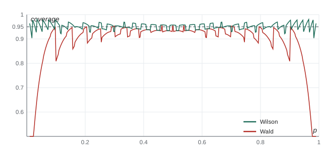
Most models have no exact pivot. The asymptotic theory of lesson 6 supplies an approximate one: \((\hat\theta - \theta)/\mathrm{se}(\hat\theta)\) is approximately standard normal, which gives the Wald interval \(\hat\theta \pm z_{\alpha/2}\,\mathrm{se}(\hat\theta)\). It is easy to compute and widely used, but its coverage can be poor. The binomial proportion is the classic example. The Wald interval \(\hat p \pm 1.96\sqrt{\hat p(1 - \hat p)/n}\) can have coverage far below 95% even for \(n\) in the hundreds when \(p\) is near 0 or 1, and its coverage oscillates erratically with \(n\) and \(p\) because the binomial is discrete. Lawrence Brown, Tony Cai and Anirban DasGupta documented this in an influential 2001 paper and recommended alternatives.

The Wilson score interval, proposed by Edwin Wilson in 1927, inverts the approximate pivot with the standard error computed at the hypothesized \(p\) rather than at \(\hat p\). Solving \(|\hat p - p| \le z\sqrt{p(1 - p)/n}\) for \(p\) gives

Its center is pulled from \(\hat p\) toward \(1/2\), it never extends outside \([0, 1]\), and its coverage stays close to 95% across almost the whole range of \(p\). The Clopper–Pearson interval of 1934 inverts exact binomial tests and guarantees coverage of at least 95%, at the cost of being conservative and wider than necessary.

Intervals and tests

There is a one-to-one correspondence between confidence sets and hypothesis tests, developed in lessons 9 and 10. A \(100(1 - \alpha)\%\) confidence set consists of exactly those values \(\theta_0\) that a level-\(\alpha\) test would not reject in a test of \(H_0: \theta = \theta_0\). The Wilson interval inverts the score test, the Wald interval inverts the Wald test, and the likelihood ratio interval of lesson 10 inverts the likelihood ratio test. This duality means that any good test gives a good interval, and an interval reports more than a single test does: it shows which parameter values are compatible with the data, not just whether one particular value is.

One-sided bounds

Sometimes only one direction matters. A regulator wants an upper bound on the failure probability of a component, and a buyer wants a lower bound on the mean lifetime of a battery. A \(100(1 - \alpha)\%\) upper confidence bound \(U(X)\) satisfies \(P_\theta(\theta \le U(X)) \ge 1 - \alpha\), and it is found from the same pivot with all of \(\alpha\) placed in one tail. For a normal mean, \(\bar X + t_{n-1, \alpha}S/\sqrt n\) is an upper bound; with \(n = 10\) and \(\alpha = 0.05\) the multiplier is \(t_{9, 0.05} = 1.833\), smaller than the two-sided 2.262. A useful special case is the rule of three: if \(n\) independent trials produce no failures, an approximate 95% upper bound for the failure probability is \(3/n\), because \((1 - p)^n \approx e^{-np}\) equals 0.05 when \(np = \log 20 \approx 3\). Thirty failure-free tests therefore support a failure probability of at most about 0.1, not zero.

Planning sample size

Confidence intervals also guide the design of a study. For a normal mean with a guessed standard deviation \(\sigma\), a 95% interval has half-width about \(1.96\sigma/\sqrt n\). To make the half-width at most \(E\), choose \(n \ge (1.96\sigma/E)^2\). For a proportion, the worst case is \(p = 1/2\), giving \(n \ge 1.96^2/(4E^2)\), about 1,068 for a margin of 0.03, which is why national opinion polls often survey about a thousand people. Halving the margin of error requires four times the sample size.

The bootstrap

For complicated statistics, such as a median, a correlation or a ratio of means, the sampling distribution may be hard to derive. Bradley Efron's bootstrap, introduced in 1979, estimates it by resampling. The idea is that the empirical distribution of the data stands in for the unknown population. Draw \(B\) samples of size \(n\) with replacement from the data, compute the statistic on each to get \(\hat\theta^*_1, \ldots, \hat\theta^*_B\), and use the spread of these values to estimate the standard error. The percentile interval takes the 2.5th and 97.5th percentiles of the bootstrap values as a 95% interval. Refinements such as the bias-corrected and accelerated (BCa) interval improve its coverage. The bootstrap needs no formula for the standard error, only a computer, but it is still an approximation: it can fail for statistics that depend on extremes, such as the sample maximum, and for very small samples.

import math, random
from statistics import mean, median, stdev

def binom_pmf(n, k, p):
    return math.comb(n, k) * p ** k * (1 - p) ** (n - k)
def wald(k, n, z=1.96):
    ph = k / n; h = z * math.sqrt(ph * (1 - ph) / n); return ph - h, ph + h
def wilson(k, n, z=1.96):
    ph = k / n; c = (ph + z * z / (2 * n)) / (1 + z * z / n)
    h = z * math.sqrt(ph * (1 - ph) / n + z * z / (4 * n * n)) / (1 + z * z / n)
    return c - h, c + h
def coverage(method, n, p):
    return sum(binom_pmf(n, k, p) for k in range(n + 1)
               if method(k, n)[0] <= p <= method(k, n)[1])

n = 30
for p in (0.05, 0.10, 0.30, 0.50):
    print(f"n=30, p={p:.2f}: Wald coverage {coverage(wald, n, p):.3f}, "
          f"Wilson coverage {coverage(wilson, n, p):.3f}")

# chi-square quantiles by bisection on the regularized lower gamma function
def gamma_cdf(x, a):
    s, term, k = 0.0, 1.0 / a, 0
    while term > 1e-15 * s or k < 5:
        s += term; k += 1; term *= x / (a + k)
    return s * math.exp(-x + a * math.log(x) - math.lgamma(a))
def chi2_upper(df, tail):
    lo, hi = 1e-9, 200.0
    for _ in range(100):
        mid = (lo + hi) / 2
        if 1 - gamma_cdf(mid / 2, df / 2) > tail: lo = mid
        else: hi = mid
    return lo
up, dn = chi2_upper(9, 0.025), chi2_upper(9, 0.975)
v = 9 * 1.8 ** 2
print(f"chi-square(9) points {up:.3f} and {dn:.3f}; sigma interval "
      f"{math.sqrt(v / up):.2f} to {math.sqrt(v / dn):.2f}")

# bootstrap percentile interval for a median
rng = random.Random(8)
data = [round(rng.lognormvariate(3, 0.6), 1) for _ in range(40)]
boots = sorted(median(rng.choices(data, k=len(data))) for _ in range(5000))
print(f"sample median {median(data):.1f}, bootstrap se {stdev(boots):.2f}, "
      f"95% percentile interval {boots[124]:.1f} to {boots[4874]:.1f}")

n=30, p=0.05: Wald coverage 0.782, Wilson coverage 0.939
n=30, p=0.10: Wald coverage 0.809, Wilson coverage 0.974
n=30, p=0.30: Wald coverage 0.953, Wilson coverage 0.930
n=30, p=0.50: Wald coverage 0.957, Wilson coverage 0.957
chi-square(9) points 19.023 and 2.700; sigma interval 1.24 to 3.29
sample median 18.0, bootstrap se 2.03, 95% percentile interval 13.4 to 20.4

The output shows the Wald interval's weakness at small \(p\): with 30 trials and \(p = 0.05\) its coverage is far below 95%, because when no successes occur the interval collapses to the single point 0. The Wilson interval stays near the nominal level, though it too oscillates a little, between about 93% and 97% at these values of \(p\), because no interval for a discrete count can have coverage exactly 95% everywhere. The chi-square points agree with the tables used in the worked example, and the bootstrap gives an interval for the median without any formula for its standard error.