From probability to statistics: samples, statistics and models

Probability runs forward. Given a model, say that each item from a production line is defective with probability 0.02 independently of the others, it tells us how the data are likely to look: how many defectives to expect in a box of 500, how variable that count is, how often it exceeds 20. Statistics runs backward. Given the data, say 14 defectives in a box of 500, it asks what we can say about the model that produced them. Is the defect rate 0.02, or has the process drifted? How precisely does one box pin the rate down? STAT-251 built the forward machinery. This course turns it around and builds the theory of inference: estimation, confidence intervals, hypothesis tests and the linear model, each derived from first principles so that we know not only which procedure to use but why it works and when it fails.

STAT-141 and STAT-151 taught many of these procedures as recipes, with software doing the arithmetic. Here we prove them. Why does the sample variance divide by \(n - 1\)? Why is the \(t\) distribution the right reference for a mean when the variance is estimated? Why is maximum likelihood so widely used, and in what precise sense is it optimal? Why does the likelihood ratio test lead to a chi-square distribution? The answers rest on the probability of lesson 1 to lesson 12 of STAT-251, especially expectation, variance, moment generating functions, transformations, the law of large numbers and the central limit theorem. Every lesson includes runnable Python that simulates the procedure, so each theorem can be checked against thousands of artificial data sets before we trust it on real ones.

Populations, samples and models

The starting point of statistical inference is a model: a family of probability distributions, one of which is assumed to have generated the data. The observations \(X_1, \ldots, X_n\) are random variables, and the numbers we record, \(x_1, \ldots, x_n\), are one realization of them. Lower case for observed values and upper case for the random variables is a convention worth keeping, because the whole subject turns on the difference: an estimate is a number, an estimator is a random variable whose distribution we can study.

The simplest and most important model is the random sample. We say \(X_1, \ldots, X_n\) are independent and identically distributed (iid) with common distribution \(F\). In a survey, this idealizes sampling with replacement from a large population, or sampling without replacement from a population so large that the difference does not matter. In a laboratory, it idealizes repeated measurement under the same conditions. In a factory, it idealizes a stable process. Whether the idealization is reasonable is a scientific question, not a mathematical one, and later lessons show how to check it. Many failures of statistics in practice are failures of this assumption: samples that are not representative, measurements that drift, observations that influence one another.

Parametric families

A parametric model is a family of distributions indexed by a parameter \(\theta\) that lives in a parameter space \(\Theta\). Examples: the Bernoulli family with \(\theta = p \in [0, 1]\), the Poisson family with \(\theta = \lambda > 0\), the normal family with \(\theta = (\mu, \sigma^2) \in \mathbb{R} \times (0, \infty)\), the exponential family of lifetimes with rate \(\lambda\). We write \(f(x; \theta)\) for the pmf or density, \(P_\theta\) and \(E_\theta\) for probabilities and expectations computed when \(\theta\) is the true value. The subscript is a reminder that every probability statement in inference is conditional on a parameter value we do not know.

A model is identifiable if different parameter values give different distributions. If two values \(\theta_1 \ne \theta_2\) produced the same distribution of the data, no amount of data could tell them apart, and asking which is true would be meaningless. Identifiability fails in less obvious ways too: in a model where \(X\) is normal with mean \(\alpha + \beta\), only the sum \(\alpha + \beta\) is identifiable. Non-parametric models make weaker assumptions, for instance only that \(F\) is continuous, and estimate features of \(F\) such as its median directly. Most of this course is parametric, because the theory is sharpest there, but the bootstrap of lesson 8 and the empirical distribution function below are non-parametric ideas.

Statistics and their sampling distributions

A statistic is any function of the data that does not depend on unknown parameters: the sample mean \(\bar X = \frac{1}{n}\sum X_i\), the sample variance \(S^2 = \frac{1}{n-1}\sum (X_i - \bar X)^2\), the sample maximum \(X_{(n)}\), the sample median, the number of observations above 10. Because a statistic is a function of random variables, it is itself a random variable, and its distribution, called its sampling distribution, describes how it would vary over repeated samples from the same population. The sampling distribution is the central object of classical inference. A procedure is judged by how it behaves over repeated samples: an estimator is good if its sampling distribution is concentrated near the true parameter, a confidence interval is valid if it covers the truth in the stated fraction of samples, and a test is sound if it rarely rejects a true hypothesis.

For the sample mean, STAT-251 already gives two key facts. If the \(X_i\) have mean \(\mu\) and variance \(\sigma^2\), linearity and independence give

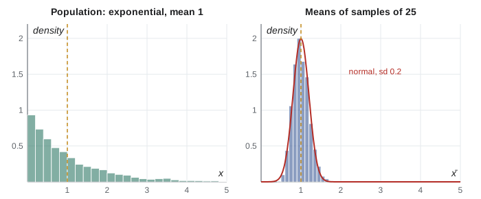
so the standard deviation of \(\bar X\), called its standard error, is \(\sigma/\sqrt n\). Quadrupling the sample size halves the standard error. And by the central limit theorem, \(\sqrt n(\bar X - \mu)/\sigma\) is approximately standard normal for large \(n\), whatever the shape of \(F\), provided the variance is finite. If the \(X_i\) are themselves normal, the distribution of \(\bar X\) is exactly \(N(\mu, \sigma^2/n)\) for every \(n\), because sums of independent normals are normal (a moment generating function argument from STAT-251 lesson 10).

The empirical distribution function

The empirical distribution function of a sample is \(\hat F_n(x) = \frac{1}{n}\#\{i : X_i \le x\}\), the fraction of observations at or below \(x\). For each fixed \(x\), \(n\hat F_n(x)\) counts successes in \(n\) independent trials with success probability \(F(x)\), so it is binomial with parameters \(n\) and \(F(x)\). Hence \(E[\hat F_n(x)] = F(x)\) and \(\operatorname{Var}(\hat F_n(x)) = F(x)(1 - F(x))/n\), and by the law of large numbers \(\hat F_n(x) \to F(x)\) with probability 1. The Glivenko–Cantelli theorem strengthens this to uniform convergence: \(\sup_x |\hat F_n(x) - F(x)| \to 0\) with probability 1. In a precise sense, a large sample reveals the whole population distribution. Many statistics are functions of \(\hat F_n\): the sample mean is the mean of \(\hat F_n\), the sample median its median. This viewpoint, plugging \(\hat F_n\) in for the unknown \(F\), is behind the method of moments in lesson 4 and the bootstrap in lesson 8.

Order statistics

Sorting the sample gives the order statistics \(X_{(1)} \le X_{(2)} \le \cdots \le X_{(n)}\). Their distributions follow from STAT-251 counting. For an iid sample from a continuous distribution with cdf \(F\) and density \(f\), the maximum satisfies \(P(X_{(n)} \le x) = P(\text{all } X_i \le x) = F(x)^n\), so its density is \(nF(x)^{n-1}f(x)\). The minimum satisfies \(P(X_{(1)} > x) = (1 - F(x))^n\). More generally, the \(k\)th order statistic has density

which we can read off as: one observation lands at \(x\), \(k - 1\) fall below and \(n - k\) above, in one of \(n!/((k-1)!\,1!\,(n-k)!)\) arrangements. Order statistics matter in reliability (a series system fails at the minimum lifetime of its parts, a parallel system at the maximum), in hydrology (the largest flood in 50 years), and in estimation, as the uniform example in lesson 3 shows.

Three questions of inference

Almost every inferential question is one of three kinds. Point estimation asks for a single best guess at \(\theta\) or at some function of it, such as a defect rate, a mean lifetime or a regression slope (lessons 3 to 7). Interval estimation asks for a range of plausible values with a stated reliability, such as a 95% confidence interval for the defect rate (lesson 8). Hypothesis testing asks whether the data are consistent with a particular claim about \(\theta\), such as the claim that the defect rate is still at its target of 0.02 (lessons 9 and 10). The linear model of lesson 11 applies all three to the relationship between a response and explanatory variables, and the capstone compares the frequentist answers with the Bayesian ones.

Two philosophies of inference run through the course. The frequentist view treats \(\theta\) as fixed and unknown and the data as random, and judges procedures by their long-run behavior over repeated samples. A 95% confidence interval is one produced by a method that covers the truth in 95 of every 100 samples. The Bayesian view treats \(\theta\) as uncertain and describes that uncertainty with a probability distribution, which Bayes' theorem updates in the light of the data. Both rest on the likelihood function introduced in lesson 5. Most of this course is frequentist, as are most published analyses, but lesson 12 shows how the Bayesian approach works and where the two agree.

import random, math
from statistics import mean, stdev

rng = random.Random(252)
mu, n, reps = 4.0, 25, 20000          # exponential population with mean 4

# one sample: estimates versus truth
x = [rng.expovariate(1 / mu) for _ in range(n)]
print(f"one sample of {n}: mean {mean(x):.3f}, sd {stdev(x):.3f}  (truth: 4, 4)")

# sampling distribution of the mean over many samples
means = [mean(rng.expovariate(1 / mu) for _ in range(n)) for _ in range(reps)]
print(f"mean of sample means {mean(means):.3f}   (theory {mu})")
print(f"sd of sample means   {stdev(means):.3f}   (theory sigma/sqrt(n) = {mu / math.sqrt(n):.3f})")

# how normal is it? fraction within 1.96 standard errors
se = mu / math.sqrt(n)
inside = sum(abs(m - mu) <= 1.96 * se for m in means) / reps
print(f"fraction within 1.96 SE: {inside:.3f}   (normal theory 0.950)")

# series system: minimum of 4 exponential lifetimes with rate 0.1
mins = [min(rng.expovariate(0.1) for _ in range(4)) for _ in range(reps)]
print(f"series system mean lifetime {mean(mins):.2f} years  (theory 2.50)")

# empirical cdf against the true cdf at a few points
big = sorted(rng.expovariate(1 / mu) for _ in range(2000))
for t in (1, 4, 10):
    Fn = sum(v <= t for v in big) / len(big)
    print(f"F_n({t:>2}) = {Fn:.3f}   F({t:>2}) = {1 - math.exp(-t / mu):.3f}")

one sample of 25: mean 3.952, sd 2.947  (truth: 4, 4)
mean of sample means 4.007   (theory 4.0)
sd of sample means   0.798   (theory sigma/sqrt(n) = 0.800)
fraction within 1.96 SE: 0.955   (normal theory 0.950)
series system mean lifetime 2.50 years  (theory 2.50)
F_n( 1) = 0.220   F( 1) = 0.221
F_n( 4) = 0.625   F( 4) = 0.632
F_n(10) = 0.915   F(10) = 0.918

The simulated standard deviation of the sample means sits close to \(\sigma/\sqrt n = 0.8\), and the fraction of means within 1.96 standard errors is close to, though a little different from, the normal value of 0.95: with \(n = 25\) the strong skew of the exponential has not quite been averaged away. The empirical cdf of 2000 observations is within a few thousandths of the true cdf at each point, an illustration of the Glivenko–Cantelli theorem.

A little history

Statistics grew from two roots. The theory of errors, developed by Legendre, Gauss and Laplace around 1800 to combine astronomical and geodetic measurements, gave least squares and the normal distribution. The study of populations, in the hands of Quetelet, Galton and Karl Pearson in the nineteenth century, gave correlation, regression and the chi-square test of fit. The modern theory of inference took shape in the early twentieth century. William Sealy Gosset, writing as Student in 1908, found the exact distribution needed for small samples. Ronald Fisher introduced maximum likelihood in papers of 1912 and 1922, along with sufficiency, efficiency and the analysis of variance. Jerzy Neyman and Egon Pearson put hypothesis testing on a decision-theoretic footing in 1933, and Neyman introduced confidence intervals in 1937. Each of these developments is the subject of a lesson in this course.