The method of moments

The method of moments is the oldest general recipe for building estimators, and still one of the most useful. Its idea is to match the theory to the data: express the population moments in terms of the parameters, replace them with the corresponding sample moments, and solve. Karl Pearson used it from the 1890s to fit his family of skewed curves to biological measurements. It is easy, it usually gives consistent estimators, and it often provides the starting point for the more efficient methods of lesson 5. This lesson develops the method, its large-sample theory through the delta method, and its limitations.

The principle

Suppose the model has \(k\) parameters \(\theta = (\theta_1, \ldots, \theta_k)\). The population moments \(\mu_j(\theta) = E_\theta[X^j]\), for \(j = 1, \ldots, k\), are functions of \(\theta\). The sample moments are \(m_j = \frac1n\sum X_i^j\). The method of moments estimator \(\tilde\theta\) solves the system

Central moments can be used instead of raw ones, and often make the algebra easier: match the mean to \(\bar X\) and the variance to \(\hat\sigma^2 = \frac1n\sum(X_i - \bar X)^2\). The justification is the law of large numbers: each \(m_j \to \mu_j(\theta)\) with probability 1, so if the map from \(\theta\) to \((\mu_1, \ldots, \mu_k)\) is one-to-one with a continuous inverse, the continuous mapping theorem gives \(\tilde\theta \to \theta\). The method of moments estimator is therefore consistent under mild conditions, a fact worth having before we know anything about efficiency.

First examples

Normal. The first two moments give \(\tilde\mu = \bar X\) and \(\tilde\sigma^2 = \hat\sigma^2\), the divide-by-\(n\) variance. Exponential with rate \(\lambda\). Since \(E[X] = 1/\lambda\), we get \(\tilde\lambda = 1/\bar X\). Poisson. \(E[X] = \lambda\) gives \(\tilde\lambda = \bar X\), but \(\operatorname{Var}(X) = \lambda\) would give \(\hat\sigma^2\) instead. Different choices of moments give different estimators. Here the mean is the better choice, as lesson 7 will show, but the ambiguity is a genuine weakness of the method.

Uniform on \([a, b]\). The mean is \((a + b)/2\) and the variance \((b - a)^2/12\). Solving gives \(\tilde a = \bar X - \sqrt{3}\hat\sigma\) and \(\tilde b = \bar X + \sqrt{3}\hat\sigma\). Here the method can give an absurd answer: \(\tilde b\) can be smaller than the largest observation, which is impossible for the true \(b\). Moment estimators do not automatically respect the support of the distribution, and for the uniform the order statistics are far better, as lesson 3 showed.

The gamma distribution

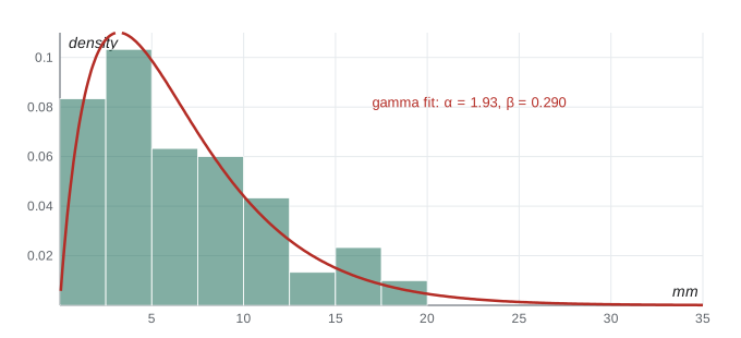
The gamma family with shape \(\alpha\) and rate \(\beta\) is a standard model for positive skewed quantities such as rainfall amounts, insurance claim sizes and service times. Its mean is \(\alpha/\beta\) and its variance \(\alpha/\beta^2\). Matching \(\bar X = \alpha/\beta\) and \(\hat\sigma^2 = \alpha/\beta^2\) and dividing gives

These have closed forms, which is a real advantage: the maximum likelihood estimator of the gamma shape solves an equation involving the digamma function and must be found numerically (lesson 5). The moment estimators are consistent, but when \(\alpha\) is small their efficiency is poor, because the sample variance of a skewed distribution is itself highly variable. A common approach in practice is to use the moment estimates as starting values for a numerical maximization of the likelihood.

Overdispersed counts

Ecologists counting organisms in quadrats, epidemiologists counting cases by district and insurers counting claims per policy often find that the variance of the counts exceeds the mean, while the Poisson model forces them to be equal. Such data are called overdispersed, and the negative binomial distribution is a common model for them. In one parameterization it has mean \(\mu\) and variance \(\mu + \mu^2/k\), where \(k > 0\) controls the extra variation and \(k \to \infty\) recovers the Poisson. Matching moments gives

provided \(\hat\sigma^2 > \bar X\). If the sample variance is below the mean, the formula gives a negative \(\tilde k\), which is outside the parameter space, and the data show no evidence of overdispersion. Moment estimators can fall outside the parameter space in small samples, and a sensible analyst then reports the boundary value, here a Poisson model, rather than a meaningless negative estimate.

Standard errors by the delta method

Moment estimators are smooth functions of sample means, so their large-sample distributions follow from the central limit theorem combined with a Taylor expansion. The delta method states that if \(\sqrt n(T_n - \theta) \to N(0, \sigma^2)\) in distribution and \(g\) is differentiable at \(\theta\) with \(g'(\theta) \ne 0\), then

The proof is one line of Taylor expansion: \(g(T_n) - g(\theta) = g'(\theta)(T_n - \theta) + o_p(|T_n - \theta|)\), and the remainder is negligible after multiplying by \(\sqrt n\). For the exponential rate, \(T_n = \bar X\) has \(\sqrt n(\bar X - 1/\lambda) \to N(0, 1/\lambda^2)\), and \(g(t) = 1/t\) has \(g'(1/\lambda) = -\lambda^2\). So \(\tilde\lambda = 1/\bar X\) is approximately normal with mean \(\lambda\) and variance \(\lambda^4 \cdot \lambda^{-2}/n = \lambda^2/n\), giving the standard error \(\tilde\lambda/\sqrt n\). For several parameters the multivariate delta method replaces \(g'\) with the gradient and \(\sigma^2\) with a covariance matrix: \(\operatorname{Var} \approx \nabla g^{\top}\Sigma\nabla g/n\).

The delta method also explains variance-stabilizing transformations. For a Poisson mean, \(\bar X\) has variance \(\lambda/n\), which depends on \(\lambda\). Choosing \(g\) with \(g'(\lambda)^2\lambda\) constant, that is \(g(\lambda) = \sqrt\lambda\), makes \(\sqrt{\bar X}\) approximately normal with variance \(1/(4n)\) whatever \(\lambda\) is. The same reasoning gives the arcsine square root transformation for proportions and the logarithm for quantities whose standard deviation is proportional to their mean.

import random, math
from statistics import mean, pvariance, stdev

rng = random.Random(252)

# gamma shape and rate by moments, repeated to see bias and spread
alpha, beta, n, reps = 2.0, 0.4, 120, 4000
a_hat, b_hat = [], []
for _ in range(reps):
    x = [rng.gammavariate(alpha, 1 / beta) for _ in range(n)]
    m, v = mean(x), pvariance(x)
    a_hat.append(m * m / v); b_hat.append(m / v)
print(f"gamma n={n}: alpha-hat mean {mean(a_hat):.3f} sd {stdev(a_hat):.3f} (true {alpha});"
      f" beta-hat mean {mean(b_hat):.3f} sd {stdev(b_hat):.3f} (true {beta})")

# negative binomial counts: mu = 3, k = 1.5, generated as a gamma-Poisson mixture
def poisson(lam):
    L, k, p = math.exp(-lam), 0, 1.0
    while True:
        p *= rng.random()
        if p < L: return k
        k += 1
mu, k = 3.0, 1.5
counts = [poisson(rng.gammavariate(k, mu / k)) for _ in range(400)]
m, v = mean(counts), pvariance(counts)
print(f"quadrat counts: mean {m:.3f}, variance {v:.3f};"
      f" k-hat = {m * m / (v - m):.3f} (true {k})" if v > m else "no overdispersion")

# delta method for the exponential rate: SE = lambda / sqrt(n)
lam, n = 0.25, 50
lam_hat = [1 / mean(rng.expovariate(lam) for _ in range(n)) for _ in range(20000)]
print(f"1/xbar: mean {mean(lam_hat):.4f} (true {lam}), sd {stdev(lam_hat):.4f},"
      f" delta-method SE {lam / math.sqrt(n):.4f}")

# variance stabilization: sd of sqrt(xbar) for several Poisson means
for lam in (1, 4, 16):
    vals = [math.sqrt(mean(poisson(lam) for _ in range(30))) for _ in range(3000)]
    print(f"Poisson lambda {lam:>2}: sd(xbar) {math.sqrt(lam / 30):.3f}, sd(sqrt xbar) {stdev(vals):.3f}"
          f" (theory {1 / math.sqrt(4 * 30):.3f})")

gamma n=120: alpha-hat mean 2.073 sd 0.326 (true 2.0); beta-hat mean 0.416 sd 0.072 (true 0.4)
quadrat counts: mean 3.038, variance 10.831; k-hat = 1.184 (true 1.5)
1/xbar: mean 0.2553 (true 0.25), sd 0.0368, delta-method SE 0.0354
Poisson lambda  1: sd(xbar) 0.183, sd(sqrt xbar) 0.093 (theory 0.091)
Poisson lambda  4: sd(xbar) 0.365, sd(sqrt xbar) 0.093 (theory 0.091)
Poisson lambda 16: sd(xbar) 0.730, sd(sqrt xbar) 0.092 (theory 0.091)

The gamma shape estimate is somewhat biased upward in samples of 120 and noticeably variable, the typical behavior of moment estimators in skewed families. The delta-method standard error for \(1/\bar X\) agrees closely with the simulated spread, and \(1/\bar X\) has a small upward bias: Jensen's inequality again, since \(1/t\) is convex. After the square root transformation, the standard deviation of the Poisson mean is about the same for every \(\lambda\), as the delta method predicts. The negative binomial \(\tilde k\) from a single sample of 400 quadrats is some way from the true 1.5: the denominator \(\hat\sigma^2 - \bar X\) is a difference of two noisy quantities, so moment estimates of a dispersion parameter are imprecise unless the sample is large.

An unstable case: the binomial with unknown n

Moment estimators can be very unstable when the parameters are hard to separate. Suppose the number of nesting pairs seen on each of several survey days is binomial with an unknown number \(N\) of pairs present and an unknown detection probability \(p\). The mean is \(Np\) and the variance \(Np(1 - p)\), so matching moments gives \(\tilde p = 1 - \hat\sigma^2/\bar X\) and \(\tilde N = \bar X/\tilde p\). When \(p\) is small the variance is nearly equal to the mean, the estimate \(\tilde p\) is a small difference of noisy quantities, and \(\tilde N\) can swing from a modest number to thousands with the addition of one more survey day, or turn negative when the sample variance happens to exceed the mean. The problem is not a defect of the method alone: the data contain little information that separates \(N\) from \(p\), because many combinations with the same product \(Np\) fit almost equally well. Lesson 5 shows that the likelihood surface for this model is a long, flat ridge, and maximum likelihood is unstable too. The honest conclusion is that such data estimate \(Np\) well and \(N\) poorly, and that a design change, such as marking individuals, is needed to estimate \(N\).

Choosing which moments to match

When there is a choice, it is usually best to match the lowest moments that identify the parameters, because sample moments of higher order are more variable and more sensitive to outliers. For location and scale parameters, the mean and variance are natural. For a parameter that governs the tail, such as the shape of a Pareto distribution of incomes or losses, the mean may not even exist for some parameter values, and moments of the logarithm, or quantiles, are safer. A related idea, the method of quantiles, equates sample and population quantiles instead of moments and is useful for heavy-tailed data.

Strengths and weaknesses

The method of moments needs only the first few moments of the model, not the full distribution, which makes it robust to some kinds of misspecification and easy to apply in complicated models. Its estimators often have closed forms. But they need not be functions of a sufficient statistic (lesson 7), so they can waste information, as the uniform example shows; the choice of moments is arbitrary; and the estimates can fall outside the parameter space. Higher sample moments are also very sensitive to outliers, since a single large observation dominates \(\sum X_i^4\). In 1982 Lars Peter Hansen generalized the idea into the generalized method of moments, which combines more moment conditions than parameters with optimal weights and became a workhorse of econometrics; it earned him a share of the 2013 economics prize in memory of Alfred Nobel.