The linear model and least squares

The linear model is the most used model in statistics. It describes how the mean of a response depends on one or more explanatory variables, and it underlies regression, analysis of variance, and much of experimental design. Its estimation method, least squares, is older than the rest of mathematical statistics: Adrien-Marie Legendre published it in 1805 in a work on the orbits of comets, and Carl Friedrich Gauss, who said he had used it since 1795, justified it in 1809 by assuming normally distributed errors, the argument that gave the normal distribution its central place. Francis Galton's studies of heredity in the 1880s gave regression its name. This lesson develops the model in matrix form, derives the least squares estimator and its properties, and connects it to the likelihood theory and tests of earlier lessons.

The model

We observe responses \(Y_1, \ldots, Y_n\) and, for each, the values of \(p\) explanatory variables collected in a row \(x_i^\top\), usually including a 1 for the intercept. The linear model states

where \(Y\) is the \(n \times 1\) response vector, \(X\) is the \(n \times p\) design matrix with rows \(x_i^\top\), \(\beta\) is a \(p \times 1\) vector of unknown coefficients and \(\varepsilon\) is a vector of uncorrelated errors with common variance. The word linear refers to the parameters, not the variables: \(Y = \beta_0 + \beta_1x + \beta_2x^2 + \varepsilon\) is a linear model, because the mean is a linear function of the \(\beta\)s, and so is a model with \(\log x\) or indicator variables for groups. We assume \(X\) has full column rank \(p\), so no explanatory variable is an exact linear combination of the others.

Least squares and the normal equations

The least squares estimator minimizes the residual sum of squares \(S(\beta) = \sum(Y_i - x_i^\top\beta)^2 = (Y - X\beta)^\top(Y - X\beta)\). Setting the gradient \(-2X^\top(Y - X\beta)\) to zero gives the normal equations

Full rank makes \(X^\top X\) invertible, and since \(S\) is a convex quadratic, this is the unique minimum. For simple regression with one explanatory variable, \(Y_i = \beta_0 + \beta_1x_i + \varepsilon_i\), the solution is

so the fitted line always passes through the point of means \((\bar x, \bar Y)\).

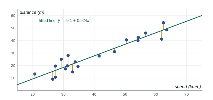
The fitted values are \(\hat Y = X\hat\beta = HY\), where \(H = X(X^\top X)^{-1}X^\top\) is called the hat matrix. Geometrically, \(H\) is the orthogonal projection onto the column space of \(X\): least squares finds the point of that subspace nearest to \(Y\). The residuals \(e = Y - \hat Y = (I - H)Y\) are orthogonal to every column of \(X\), so they sum to zero when there is an intercept and are uncorrelated with each explanatory variable in the sample. Since \(H\) is symmetric and idempotent with trace \(p\), the residual vector lives in a space of dimension \(n - p\).

Properties of the estimator

Because \(\hat\beta = (X^\top X)^{-1}X^\top Y\) is linear in \(Y\), its mean and covariance follow directly from those of \(Y\):

For simple regression, \(\mathrm{Var}(\hat\beta_1) = \sigma^2/S_{xx}\): the slope is estimated more precisely when the \(x\) values are spread out, which is a lesson for design. The Gauss–Markov theorem states that among all linear unbiased estimators of \(\beta\), least squares has the smallest variance; it is the best linear unbiased estimator (BLUE). Gauss proved it in 1821 to 1823, and Andrey Markov's later textbook treatment attached his name. The theorem needs only uncorrelated errors with equal variance, not normality, but it restricts attention to linear estimators; with heavy-tailed errors, non-linear robust methods can do much better.

The error variance is estimated from the residuals:

which is unbiased for \(\sigma^2\), since \(E[\mathrm{RSS}] = \sigma^2\,\mathrm{tr}(I - H) = \sigma^2(n - p)\). Dividing by \(n - p\) rather than \(n\) generalizes the \(n - 1\) of the sample variance: one degree of freedom is used for each estimated coefficient.

Normal errors: likelihood, t and F

If the errors are also normal, \(\varepsilon \sim N(0, \sigma^2 I)\), the log-likelihood is \(-\frac n2\log(2\pi\sigma^2) - S(\beta)/(2\sigma^2)\), so the MLE of \(\beta\) is exactly the least squares estimator, as Gauss observed. The MLE of \(\sigma^2\) is \(\mathrm{RSS}/n\), biased like the normal variance MLE of lesson 5. Moreover, \(\hat\beta \sim N(\beta, \sigma^2(X^\top X)^{-1})\), \((n - p)s^2/\sigma^2 \sim \chi^2_{n-p}\), and the two are independent, by the same argument as for \(\bar X\) and \(S^2\). Hence for each coefficient

which gives exact \(t\) tests of \(\beta_j = 0\) and confidence intervals \(\hat\beta_j \pm t_{n-p, \alpha/2}\,\mathrm{se}(\hat\beta_j)\).

To test whether several coefficients are zero at once, compare a reduced model with \(q\) fewer parameters against the full model. With residual sums of squares \(\mathrm{RSS}_0\) and \(\mathrm{RSS}_1\),

This \(F\) test is the likelihood ratio test of lesson 10: \(\Lambda = (\mathrm{RSS}_1/\mathrm{RSS}_0)^{n/2}\) is a decreasing function of \(F\), and the exact \(F\) distribution replaces the chi-square approximation. Fisher developed the analysis of variance in the 1920s from this decomposition. With one restriction, \(F = t^2\).

Estimating a mean response and predicting a new one

Two questions about a new point \(x_0\) are easily confused. The first asks for the mean response there, \(x_0^\top\beta\), estimated by \(x_0^\top\hat\beta\) with variance \(\sigma^2x_0^\top(X^\top X)^{-1}x_0\). The second asks where a single new observation \(Y_0 = x_0^\top\beta + \varepsilon_0\) is likely to fall. Its prediction error \(Y_0 - x_0^\top\hat\beta\) includes the new error \(\varepsilon_0\) as well as the estimation error, so its variance is \(\sigma^2[1 + x_0^\top(X^\top X)^{-1}x_0]\). For simple regression the two intervals are

Both are narrowest at \(\bar x\) and widen as \(x_0\) moves away, which is a warning against extrapolation. As \(n\) grows, the confidence interval for the mean shrinks to a point, but the prediction interval never becomes narrower than about \(\pm 1.96\sigma\), because individual outcomes keep their own randomness. In the worked example of this lesson, at \(x_0 = 3\) the two half-widths are \(3.182 \times 0.730 \times \sqrt{0.2} \approx 1.04\) and \(3.182 \times 0.730 \times \sqrt{1.2} \approx 2.54\).

Fit and diagnostics

The coefficient of determination \(R^2 = 1 - \mathrm{RSS}/\sum(Y_i - \bar Y)^2\) is the proportion of the variation in \(Y\) explained by the model. It always increases when variables are added, even useless ones, so the adjusted version \(1 - (1 - R^2)(n - 1)/(n - p)\) or a criterion such as AIC is better for comparing models of different sizes. A high \(R^2\) does not show that the model is correct, and a low one does not make it useless.

The assumptions are checked mainly with residuals. A plot of residuals against fitted values should show no pattern; curvature suggests a missing term, and a funnel shape suggests variance that grows with the mean, which a log transformation may cure. A normal quantile plot of residuals checks the normality needed for exact \(t\) and \(F\) tests, though with moderate \(n\) the central limit theorem makes those tests robust to mild departures. The diagonal entries \(h_{ii}\) of the hat matrix, called leverages, measure how far each observation's explanatory values are from the rest; they average \(p/n\), and an observation with high leverage and a large residual can dominate the fit. Cook's distance, proposed by Dennis Cook in 1977, combines the two to measure each observation's influence.

Correlation between explanatory variables, called collinearity, does not bias \(\hat\beta\) but inflates its variance through \((X^\top X)^{-1}\), making individual coefficients unstable even when the fit as a whole is good. And regression shows association, not causation: a coefficient measures how the mean of \(Y\) differs between units with different \(x\), holding the other included variables fixed, not what would happen if \(x\) were changed, unless the \(x\) values were assigned at random.

import random
from statistics import mean

def solve(A, b):                         # Gauss-Jordan elimination
    n = len(A); M = [row[:] + [bi] for row, bi in zip(A, b)]
    for c in range(n):
        piv = max(range(c, n), key=lambda r: abs(M[r][c])); M[c], M[piv] = M[piv], M[c]
        for r in range(n):
            if r != c:
                f = M[r][c] / M[c][c]
                M[r] = [a - f * bb for a, bb in zip(M[r], M[c])]
    return [M[i][n] / M[i][i] for i in range(n)]
def inverse(A):
    n = len(A)
    cols = [solve(A, [1.0 if i == j else 0.0 for i in range(n)]) for j in range(n)]
    return [[cols[j][i] for j in range(n)] for i in range(n)]
def ols(X, y):
    p = len(X[0])
    XtX = [[sum(r[i] * r[j] for r in X) for j in range(p)] for i in range(p)]
    Xty = [sum(r[i] * yi for r, yi in zip(X, y)) for i in range(p)]
    b = solve(XtX, Xty)
    rss = sum((yi - sum(bj * xj for bj, xj in zip(b, r))) ** 2 for r, yi in zip(X, y))
    return b, rss, inverse(XtX)

# the worked example
b, rss, V = ols([[1, x] for x in (1, 2, 3, 4, 5)], [3, 5, 6, 9, 12])
s2 = rss / 3
print(f"worked example: b0 {b[0]:.3f}, b1 {b[1]:.3f}, RSS {rss:.3f}, se(b1) {(s2 * V[1][1]) ** 0.5:.3f}")

# simulated data: y = 2 + 1.5 x1 + 0 x2 + noise, with x1 and x2 correlated
rng = random.Random(2)
n = 60
x1 = [rng.uniform(0, 10) for _ in range(n)]
x2 = [0.6 * a + rng.gauss(0, 2) for a in x1]
y = [2 + 1.5 * a + rng.gauss(0, 3) for a in x1]
X1 = [[1, a, c] for a, c in zip(x1, x2)]
b, rss1, V = ols(X1, y)
s2 = rss1 / (n - 3)
for name, bj, vjj in zip(("intercept", "x1", "x2"), b, (V[0][0], V[1][1], V[2][2])):
    se = (s2 * vjj) ** 0.5
    print(f"{name:9s} estimate {bj:7.3f}  se {se:.3f}  t {bj / se:6.2f}")
b0, rss0, _ = ols([[1] for _ in range(n)], y)        # intercept-only model
F = ((rss0 - rss1) / 2) / (rss1 / (n - 3))
r2 = 1 - rss1 / rss0
print(f"F test of x1 = x2 = 0: F = {F:.1f} on 2 and {n - 3} df; R^2 = {r2:.3f}")

worked example: b0 0.400, b1 2.200, RSS 1.600, se(b1) 0.231
intercept estimate   2.015  se 0.811  t   2.49
x1        estimate   1.497  se 0.189  t   7.90
x2        estimate  -0.019  se 0.209  t  -0.09
F test of x1 = x2 = 0: F = 68.6 on 2 and 57 df; R^2 = 0.707

The solver reproduces the hand calculation. In the simulated data, the coefficient of \(x_1\) is close to its true value of 1.5 with a large \(t\) statistic, while the coefficient of \(x_2\), whose true value is zero, has a small \(t\) statistic even though \(x_2\) is correlated with the response through \(x_1\). The \(F\) test of both slopes together is overwhelming. This is the multiple regression idea at work: each coefficient measures the effect of its variable with the others held fixed.