Properties of maximum likelihood estimators

Lesson 5 showed how to compute maximum likelihood estimates. This lesson explains why they are trusted. Under regularity conditions that hold for most textbook models, the MLE is consistent, approximately normal in large samples, and asymptotically efficient: no other reasonable estimator has smaller variance in the limit. These results, sketched by Fisher in 1922 and 1925 and made rigorous by Cramér in his 1946 book Mathematical Methods of Statistics, give every MLE an approximate standard error and confidence interval, computed from the curvature of the log-likelihood. They are the reason almost every statistical package reports a standard error next to each estimate.

The score and Fisher information

For one observation with density \(f(x; \theta)\), the score is \(U(\theta) = \frac{\partial}{\partial\theta}\log f(X; \theta)\). Under regularity conditions that allow differentiation under the integral sign, the score has mean zero at the true parameter value:

Its variance is the Fisher information. Differentiating the identity a second time gives an equivalent formula, often easier to compute:

For an iid sample of size \(n\), the scores add, so the information in the sample is \(nI(\theta)\). Information is a measure of how sharply the log-likelihood is expected to curve near the true value, which matches the picture from lesson 5: more data, more curvature, more information.

Standard cases. Bernoulli: \(\log f = x\log p + (1 - x)\log(1 - p)\), second derivative \(-x/p^2 - (1 - x)/(1 - p)^2\), with expected value \(-1/p - 1/(1 - p)\), so \(I(p) = 1/[p(1 - p)]\). Poisson: \(\log f = x\log\lambda - \lambda - \log x!\), second derivative \(-x/\lambda^2\), so \(I(\lambda) = 1/\lambda\). Exponential with rate \(\lambda\): \(\log f = \log\lambda - \lambda x\), so \(I(\lambda) = 1/\lambda^2\). Normal mean with known \(\sigma^2\): \(I(\mu) = 1/\sigma^2\). In each case \(1/(nI)\) turns out to be the variance, or approximate variance, of the MLE.

Consistency

Why should maximizing the likelihood find the true parameter? Divide the log-likelihood by \(n\). By the law of large numbers, \(\frac1n\ell(\theta) \to E_{\theta_0}[\log f(X; \theta)]\) for each \(\theta\), where \(\theta_0\) is the true value. By Jensen's inequality,

with equality only when the two densities agree. The negative of the left side is the Kullback–Leibler divergence of \(f(\cdot; \theta)\) from \(f(\cdot; \theta_0)\). So the limiting average log-likelihood is uniquely maximized at \(\theta_0\), provided the parameter is identifiable, meaning different values give different distributions. Turning this into a proof that \(\hat\theta \to \theta_0\) in probability needs some uniformity of the convergence, which Wald supplied in 1949, but the idea is just this: in the long run, the true parameter fits the data best on average.

Asymptotic normality

Expand the score around the true value. Since \(\ell'(\hat\theta) = 0\),

The numerator is \(n^{-1/2}\) times a sum of iid scores with mean 0 and variance \(I(\theta_0)\), so by the central limit theorem it converges in distribution to \(N(0, I(\theta_0))\). The denominator is an average of iid terms with mean \(I(\theta_0)\), so by the law of large numbers it converges in probability to \(I(\theta_0)\). Slutsky's theorem, which says that if \(Y_n \to Y\) in distribution and \(c_n \to c\) in probability then \(Y_n/c_n \to Y/c\), combines the two:

In words, for large \(n\) the MLE is approximately normal, centered on the truth, with variance \(1/(nI(\theta_0))\). The regularity conditions behind the sketch are that the support does not depend on \(\theta\), the true value is in the interior of \(\Theta\), the log-density has enough continuous derivatives, and the information is finite and positive. The uniform on \([0, \theta]\) fails the first condition, and there the MLE \(X_{(n)}\) converges at rate \(1/n\), not \(1/\sqrt n\), with an exponential limit rather than a normal one.

Standard errors and Wald intervals

The asymptotic variance involves the unknown \(\theta_0\), so in practice it is estimated, either by plugging in, \(1/(nI(\hat\theta))\), or by the observed information \(J(\hat\theta) = -\ell''(\hat\theta)\), the actual curvature of the log-likelihood at its peak. Efron and Hinkley argued in 1978 that the observed information is often the better choice, because it reflects the data actually seen. Either way, the standard error is

and an approximate 95% confidence interval is \(\hat\theta \pm 1.96\,\mathrm{se}(\hat\theta)\), called the Wald interval after Abraham Wald. For a proportion this gives \(\hat p \pm 1.96\sqrt{\hat p(1 - \hat p)/n}\), the familiar interval of introductory courses. Lesson 8 shows that the Wald interval can perform badly when \(n\) is small or the estimate is near a boundary, and lesson 10 gives the likelihood ratio interval, which is usually better.

Functions of the MLE

By invariance, \(g(\hat\theta)\) is the MLE of \(g(\theta)\), and the delta method of lesson 4 gives its approximate variance, \(g'(\theta)^2/(nI(\theta))\). For the help desk, the probability of a call-free hour is \(e^{-\lambda}\); its MLE is \(e^{-7.8} \approx 0.00041\), with standard error \(e^{-7.8} \times 0.442 \approx 0.00018\). The same result follows from reparameterizing: information transforms as \(I_\eta(\eta) = I_\theta(\theta)/g'(\theta)^2\) when \(\eta = g(\theta)\). Because the normal approximation is better on some scales than others, intervals are often computed on a transformed scale, such as the log of a rate or the logit of a probability, and transformed back, which keeps them inside the parameter space.

Several parameters

With a parameter vector \(\theta = (\theta_1, \ldots, \theta_k)\), the score is the gradient vector and the Fisher information is the \(k \times k\) matrix with entries \(I_{jk} = -E[\partial^2\log f/\partial\theta_j\partial\theta_k]\). The MLE is asymptotically multivariate normal with covariance matrix \(I(\theta)^{-1}/n\). For the normal model with parameters \(\mu\) and \(\sigma^2\),

so \(\hat\mu\) and \(\hat\sigma^2\) are asymptotically uncorrelated, with variances \(\sigma^2/n\) and \(2\sigma^4/n\). The off-diagonal zero says that not knowing \(\sigma^2\) costs nothing in estimating \(\mu\), in large samples. When the information matrix has non-zero off-diagonal entries, as for the gamma shape and rate, the standard error of one parameter is larger when the other is estimated than when it is known: the correct variance is a diagonal entry of the inverse matrix, not the inverse of a diagonal entry. Ignoring this is a common way to understate uncertainty.

Efficiency

Lesson 7 proves the Cramér–Rao inequality: under the same regularity conditions, any unbiased estimator of \(\theta\) has variance at least \(1/(nI(\theta))\). The MLE attains this bound asymptotically, so in large samples it is as precise as any unbiased estimator can be. This is the sense in which Fisher called the MLE efficient, and it is why the moment estimators of lesson 4 are usually used only as starting values. The asymptotic relative efficiency of an estimator is the ratio \(1/(nI)\) to its asymptotic variance. For the gamma shape with \(\alpha = 2\), the method of moments has asymptotic efficiency of only about 0.58, and it falls further as \(\alpha\) decreases, to about 0.39 at \(\alpha = 1\).

The phrase in large samples hides a subtlety. Joseph Hodges found in 1951 an estimator of a normal mean that equals \(\bar X\) except that it is replaced by 0 whenever \(|\bar X| < n^{-1/4}\). At \(\mu = 0\) its asymptotic variance is zero, beating the bound, and at every other \(\mu\) it matches \(\bar X\). Lucien Le Cam showed in 1953 that such superefficiency can occur only on a set of parameter values of measure zero, and that the price is poor behavior for \(\mu\) near 0 at any fixed \(n\). The modern statement of the MLE's optimality is therefore about estimators that behave regularly near every parameter value, not about each point separately.

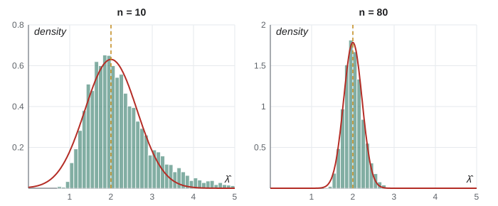
A caution about the word asymptotic. The approximations are limits as \(n \to \infty\); for a particular sample size they may be good or poor. The simulation below shows how close they are for an exponential rate.

import math, random
from statistics import mean, pvariance

rng = random.Random(6)
lam = 2.0
for n in (10, 80):
    mles = [1 / mean(rng.expovariate(lam) for _ in range(n)) for _ in range(4000)]
    crlb = lam ** 2 / n                      # 1 / (n I(lambda)), I = 1 / lambda^2
    print(f"n = {n:2d}: mean MLE {mean(mles):.3f}, var {pvariance(mles):.4f}, "
          f"1/(nI) {crlb:.4f}, ratio {pvariance(mles) / crlb:.2f}")

# coverage of the Wald interval  lambda-hat +/- 1.96 lambda-hat / sqrt(n)
for n in (10, 80):
    low = high = 0
    for _ in range(4000):
        lh = 1 / mean(rng.expovariate(lam) for _ in range(n))
        se = lh / math.sqrt(n)
        low += lam < lh - 1.96 * se          # interval entirely above the truth
        high += lam > lh + 1.96 * se         # interval entirely below the truth
    print(f"n = {n:2d}: Wald coverage {1 - (low + high) / 4000:.3f}, "
          f"misses above {low / 4000:.3f}, below {high / 4000:.3f}")

# help desk example
n, total = 40, 312
lh = total / n; se = math.sqrt(lh / n)
print(f"help desk: rate {lh:.2f}, se {se:.3f}, interval {lh - 1.96 * se:.2f} to {lh + 1.96 * se:.2f}")
print(f"P(no calls) MLE {math.exp(-lh):.5f}, delta-method se {math.exp(-lh) * se:.5f}")

n = 10: mean MLE 2.230, var 0.6197, 1/(nI) 0.4000, ratio 1.55
n = 80: mean MLE 2.018, var 0.0529, 1/(nI) 0.0500, ratio 1.06
n = 10: Wald coverage 0.958, misses above 0.005, below 0.037
n = 80: Wald coverage 0.954, misses above 0.019, below 0.027
help desk: rate 7.80, se 0.442, interval 6.93 to 8.67
P(no calls) MLE 0.00041, delta-method se 0.00018

With 10 observations, the MLE of the rate is noticeably biased upward and its variance is well above \(1/(nI)\), since \(1/\bar X\) has a right-skewed distribution; the Wald interval's overall coverage happens to be close to 95%, but its misses are lopsided, falling mostly on one side of the truth, so its two tails are not the 2.5% each that a 95% interval promises. With 80 observations, the bias is small, the variance ratio is close to 1 and the misses are more evenly split. This pattern is typical: asymptotic results are reliable for moderate samples in well-behaved models, and checking them by simulation, as here, is cheap and good practice.

When the model is wrong

All of these results assume the model is correct. In practice it is at best an approximation, and the MLE then converges to the parameter value whose distribution is closest to the truth in Kullback–Leibler divergence, by the same Jensen argument used for consistency. Peter Huber showed in 1967 that the MLE is still asymptotically normal in this case, but its variance is no longer \(1/(nI)\). The correct variance has the sandwich form \(A^{-1}BA^{-1}/n\), where \(A\) is minus the expected second derivative of the log-density and \(B\) is the variance of the score, both computed under the true distribution. When the model is right, \(A = B = I\) and the sandwich collapses to the usual formula. Halbert White popularized the estimated version for regression in 1980 and 1982, and it is the source of the robust standard errors reported by econometrics software. A large gap between model-based and sandwich standard errors is a useful sign that the model is missing something, such as overdispersion in count data, where the Poisson variance \(\lambda\) is smaller than the actual variance.