
ROB-460 · Lesson 11 of 12 · 32 min
Communication, autonomy and supervision in the field
Field robots operate where networks are weak, intermittent or absent, and often with one person supervising several machines from far away. How a robot communicates shapes how much autonomy it needs, and how much autonomy it has shapes how many robots a person can supervise. This lesson covers the radio and satellite links used in the field, link budgets and propagation, relays and mesh networks, delay- and disruption-tolerant networking, frameworks for describing levels of autonomy, the workload of supervising fleets, and fault management. ROB-430 lesson 6 treated teleoperation and shared autonomy at the level of a single operator and robot; here the focus is on networks and fleets.
Communication options in the field
No single technology covers every field situation, so robots often carry two or three radios. Wi-Fi in license-exempt bands gives high bandwidth over short ranges and is cheap, but range outdoors is limited to hundreds of meters without directional antennas. Mesh radios, including military-style mobile ad hoc network (MANET) radios and mesh Wi-Fi, route traffic through intermediate nodes so that robots can relay for each other. Private LTE and 5G networks give wide-area coverage with managed quality of service and are used in mines, ports and large farms. Low-power wide-area technologies such as LoRa carry small telemetry messages over kilometers with very low power. Satellite links reach anywhere with sky view: geostationary services have high latency of around 600 ms round trip; low-earth-orbit constellations such as Starlink provide broadband with latencies of tens of milliseconds and have transformed connectivity at remote sites since about 2021; Iridium's network provides global low-rate messaging and voice, including in polar regions, and is widely used for telemetry from gliders, floats and Arctic equipment.
| Technology | Typical range | Typical data rate | Field uses |
|---|---|---|---|
| Wi-Fi (2.4 or 5 GHz) | 100 to 500 m outdoors; more with directional antennas | Tens to hundreds of Mb/s | Local data offload, short-range video |
| Mesh and MANET radios | Hundreds of meters to km per hop | Mb/s to tens of Mb/s | Robot teams, relays in tunnels and valleys |
| Private LTE or 5G | Kilometers per cell | Tens to hundreds of Mb/s | Mines, ports, large sites |
| LoRa and similar | Several km | Hundreds of b/s to tens of kb/s | Low-power telemetry, sensor networks |
| LEO satellite broadband | Global where licensed, needs sky view | Tens to hundreds of Mb/s | Remote site backhaul, supervision |
| Iridium messaging | Global including poles | Bytes to kilobytes per message | Status of gliders, floats, Arctic robots |
In the United States, radio equipment must be authorized under Federal Communications Commission (FCC) rules; license-exempt devices operate under Part 15, and private LTE networks commonly use the Citizens Broadband Radio Service in the 3.5 GHz band or other licensed spectrum. Satellite services must be authorized by the FCC.
Link budgets and propagation
Whether a link works is decided by its link budget: the received power must exceed the receiver's sensitivity by a margin that covers fading. The received power in decibels is the transmit power plus antenna gains minus losses. The largest loss is usually free-space path loss, which for distance \( d \) in kilometers and frequency \( f \) in megahertz is
Free-space loss rises by 6 dB each time distance doubles, and by 6 dB each time frequency doubles for antennas of fixed gain. Field links suffer additional losses from vegetation, terrain and obstacles. Radio waves need a clear region around the direct line, the first Fresnel zone, whose radius at the midpoint of a path of length \( d \) is \( r = \tfrac{1}{2}\sqrt{\lambda d} \); if the ground, crops or trees intrude into more than about 40 percent of it, losses rise sharply. Lower frequencies diffract around obstacles and penetrate foliage better, which is why 900 MHz radios are popular for long-range farm and forestry telemetry, while 5 GHz links need clear line of sight.
# Link budgets for a field robot at 1.5 km in three bands (illustrative equipment values)
import math
def fspl_db(d_km, f_mhz):
    return 20 * math.log10(d_km) + 20 * math.log10(f_mhz) + 32.44
def fresnel_mid_m(d_km, f_mhz):
    lam = 299.792458 / f_mhz          # wavelength in m
    return 0.5 * math.sqrt(lam * d_km * 1000)
links = {   # f (MHz), tx dBm, antenna gains dBi (each end), rx sensitivity dBm, foliage loss dB at 1.5 km
    "900 MHz telemetry": (915, 30, 3, -110, 8),
    "2.4 GHz mesh":      (2440, 27, 5, -90, 18),
    "5.8 GHz Wi-Fi":     (5800, 25, 8, -80, 30),
}
d = 1.5
for name, (f, ptx, g, sens, foliage) in links.items():
    loss = fspl_db(d, f)
    for veg in (0, foliage):
        prx = ptx + 2 * g - loss - veg
        print(f"{name:18s} {'with trees' if veg else 'clear LOS ':10s} FSPL {loss:5.1f} dB  "
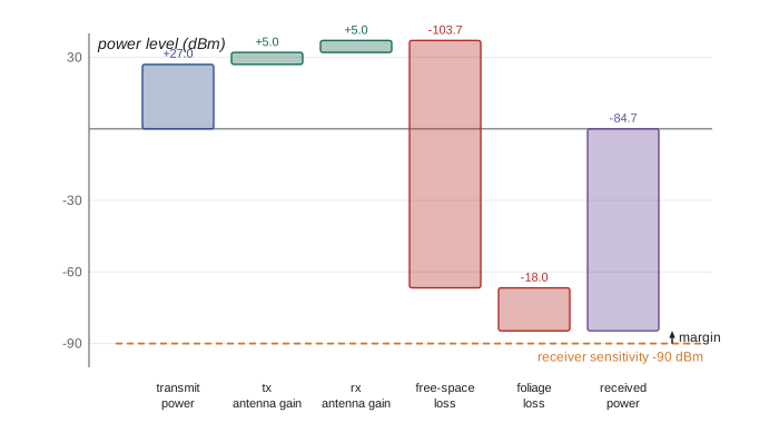
f"rx {prx:6.1f} dBm margin {prx - sens:5.1f} dB Fresnel radius {fresnel_mid_m(d, f):4.1f} m")900 MHz telemetry clear LOS FSPL 95.2 dB rx -59.2 dBm margin 50.8 dB Fresnel radius 11.1 m 900 MHz telemetry with trees FSPL 95.2 dB rx -67.2 dBm margin 42.8 dB Fresnel radius 11.1 m 2.4 GHz mesh clear LOS FSPL 103.7 dB rx -66.7 dBm margin 23.3 dB Fresnel radius 6.8 m 2.4 GHz mesh with trees FSPL 103.7 dB rx -84.7 dBm margin 5.3 dB Fresnel radius 6.8 m 5.8 GHz Wi-Fi clear LOS FSPL 111.2 dB rx -70.2 dBm margin 9.8 dB Fresnel radius 4.4 m 5.8 GHz Wi-Fi with trees FSPL 111.2 dB rx -100.2 dBm margin -20.2 dB Fresnel radius 4.4 m
In clear line of sight all three links close with margin, but through trees the 5.8 GHz link fails, the 2.4 GHz link keeps only about 5 dB, less than a prudent fade margin, and 900 MHz still has a healthy margin of more than 40 dB. The trade-off is bandwidth: the low-frequency telemetry link carries tens of kilobits per second, enough for status and commands but not for video. A common field design uses a low-rate, long-range link for safety-critical commands and status, and a high-rate link for video and data when available. Fade margins of 10 to 20 dB are typical in planning because multipath and moving vegetation cause the received signal to fluctuate.
Worked problem
Fresnel clearance over a crop field
A base station and a robot 2 km apart communicate at 2.4 GHz with antennas 3 m high over flat ground. Maize grows to 2.5 m. Is the first Fresnel zone adequately clear at the midpoint?
Show solution
- Wavelength: \( \lambda = 300 / 2440 \approx 0.123 \) m.
- Midpoint radius: \( r = 0.5\sqrt{0.123 \times 2000} \approx 7.8 \) m.
- The direct line is 3 m above the ground; the zone extends 7.8 m below it, far into the ground and the crop.
- 60 percent clearance needs about 4.7 m of free space below the line, so the antennas would need to be roughly 2.5 + 4.7 = 7.2 m high.
Answer: No: the Fresnel zone is heavily obstructed, so expect large extra losses; raising the base antenna on a mast, using a lower frequency or adding relays would help.
Relays, mesh networks and breadcrumbs
When direct links fail, robots can carry the network with them. In tunnels, mines and valleys, robots drop small relay radios, often called breadcrumbs, at points where the signal from the last relay weakens, maintaining a chain back to the base. Teams in the DARPA Subterranean Challenge used this widely, with ground robots carrying several relays and deploying them by monitoring signal strength. Robots can also act as mobile relays: a drone hovering above a valley or a ground robot parked on a ridge extends coverage for the others. Lesson 10's algebraic connectivity applies here too: planners can position relays to keep the communication graph connected and, ideally, to maximize its connectivity so that one failure does not split the network.
Mesh networks route traffic dynamically, but every hop adds latency and shares the radio channel, so throughput falls with the number of hops. Robots must prioritize traffic: safety commands and heartbeats first, then status and compressed maps, then imagery and logs. Heartbeat messages let each robot detect loss of link, and a clear policy for what to do on link loss, for example stop, continue the current task, return to the last point of good signal or proceed to a rally point, is part of every field robot's safety case.
Delay- and disruption-tolerant networking
Conventional internet protocols assume a continuous end-to-end path with short delays. In space, underwater and in many field deployments, such paths exist only intermittently. Delay- and disruption-tolerant networking (DTN) uses store-carry-forward: nodes store data until a link is available, and may physically carry it, as when a data mule robot drives from a remote work area to a base and uploads what it has collected. The Bundle Protocol, standardized by the IETF in RFC 9171 in 2022 as version 7, provides this at the network level, with custody transfer so that responsibility for a bundle passes from node to node. NASA has tested DTN on the International Space Station and plans it for lunar communications, and similar ideas are used in underwater networks, where vehicles exchange data when they meet or surface.
Worked problem
Planning a data mule
Three survey robots each collect 40 GB per day in a valley with no network. A data mule robot can drive to them, download at 200 Mb/s over Wi-Fi when within 50 m, and return to a base with satellite backhaul at 50 Mb/s. How long does the mule spend downloading each day, and how long does the upload take?
Show solution
- Total data: \( 3 \times 40 = 120 \) GB = 960 Gb.
- Download time: \( 960 / 0.2 = 4800 \) s, about 80 min plus driving.
- Upload time: \( 960 / 0.05 = 19200 \) s, about 5.3 h.
- If the upload cannot finish daily, the robots should compress or prioritize data, or the base should store data for physical collection.
Answer: About 80 minutes of downloads and over 5 hours of satellite upload per day; prioritizing summaries and sending raw data later keeps the most important information flowing.
Levels of autonomy
Several frameworks describe how much a robot decides for itself. Sheridan and Verplank's 1978 scale runs from level 1, where the computer offers no assistance and the human does everything, to level 10, where the computer decides everything and ignores the human, with intermediate levels such as suggesting alternatives, executing if the human approves, and informing the human after acting. For automated road vehicles, SAE J3016 defines levels 0 to 5, which ROB-420 lesson 1 described. The US National Institute of Standards and Technology's Autonomy Levels for Unmanned Systems (ALFUS) framework rates autonomy along three axes: the complexity of the mission, the difficulty of the environment and the independence from humans. That three-axis view suits field robots well: a robot may be highly autonomous for driving down a known orchard row but need human approval for crossing a road or entering a new field.
In practice, field robots use adjustable or sliding autonomy, in which the level changes with the situation. A survey drone flies its mission autonomously, asks the operator to confirm a landing site if wind exceeds a threshold, and lets the operator take manual control during an emergency. Designers decide which decisions require human approval, which the robot reports afterwards, and which it never reports, and they record those decisions in the concept of operations and the safety case.
| Sheridan level (selected) | What the computer does | Field example |
|---|---|---|
| 1 | Offers no assistance; the human acts | Manual remote control of a demining robot |
| 4 | Suggests one alternative | System proposes a route around a flooded area for operator selection |
| 5 | Executes the suggestion if the human approves | Robot crosses a field boundary after operator confirmation |
| 7 | Executes automatically, then informs the human | AUV changes depth to avoid a detected obstacle and reports it |
| 9 | Informs the human only if it decides to | Routine path adjustments not reported |
| 10 | Decides everything, ignoring the human | Generally unacceptable for field robots that may affect people |
Supervising fleets
How many robots can one person supervise? Olsen and Goodrich proposed that the fan-out of a supervisor, the number of robots one person can manage, depends on how long a robot can be neglected before its performance degrades (neglect time, NT) and how long each interaction takes (interaction time, IT). A simple estimate is
The estimate is optimistic because it ignores the time to switch attention between robots and to regain situation awareness, and because interventions tend to cluster: several robots may need help at once when the weather changes or a network fails. Still, it shows the two levers. Better autonomy increases neglect time; better interfaces and tools reduce interaction time. Mining control rooms supervising autonomous haul fleets, farm operators watching several machines on a tablet and DARPA SubT supervisors managing mixed teams all rely on interfaces that summarize fleet status, raise prioritized alerts and let the operator act with a few high-level commands.
# Fan-out and queueing: how many robots can one supervisor handle?
import numpy as np
rng = np.random.default_rng(11)
def simulate(n_robots, mean_neglect_min, mean_interact_min, shift_min=480, trials=300):
    waits = []
    for _ in range(trials):
        events = []
        for r in range(n_robots):
            t = rng.exponential(mean_neglect_min)
            while t < shift_min:
                events.append(t)
                t += mean_interact_min + rng.exponential(mean_neglect_min)
        events.sort()
        free_at, total_wait = 0.0, 0.0
        for t in events:                       # one supervisor serves requests in order
            start = max(t, free_at)
            total_wait += start - t
            free_at = start + rng.exponential(mean_interact_min)
        waits.append(total_wait / max(len(events), 1))
    return np.mean(waits)
NT, IT = 40.0, 4.0
print(f"simple fan-out estimate: {NT / IT + 1:.0f} robots")
for n in (4, 8, 11, 14):
print(f"{n:2d} robots: average wait for the supervisor {simulate(n, NT, IT):5.1f} min")simple fan-out estimate: 11 robots 4 robots: average wait for the supervisor 1.8 min 8 robots: average wait for the supervisor 8.5 min 11 robots: average wait for the supervisor 26.6 min 14 robots: average wait for the supervisor 76.6 min
The simple formula suggests eleven robots, but the simulation shows that waiting times rise steeply well before that point, because requests arrive randomly and queue. Robots waiting for help are idle, so the practical fan-out depends on how costly that idle time is; many operations plan for a supervisor to be busy no more than about half the time so that bursts of requests can be absorbed.
Fault management and safe modes
Because help is far away, field robots need layered fault management. Health monitoring checks sensors, actuators, temperatures, battery state and software processes, and detects degraded performance such as rising wheel slip or localization uncertainty. Fault responses range from local recovery (restart a process, switch to a backup sensor), through degraded operation (slow down, use a simpler behavior), to a safe mode in which the robot stops or moves to a safe location, maintains power and communication, and waits for instructions. Spacecraft pioneered this approach, with safe modes that point solar panels at the Sun and antennas at Earth; field robots adapt it to their environments, for example an AUV that drops a weight and surfaces, or a farm robot that stops, raises its implement and calls for help. Cybersecurity is part of the same picture: links and remote supervision interfaces are attack surfaces, and ROB-450 lesson 10 explained how security failures can defeat safety functions.
Common mistakes
MistakeAssuming a radio's advertised range will be achieved in the field.
InsteadCompute a link budget with vegetation, terrain and Fresnel clearance, and add a fade margin of 10 to 20 dB.
MistakeSending video and safety commands over the same congested link without priorities.
InsteadPrioritize safety commands and heartbeats, and use a separate robust link for them where possible.
MistakeLeaving the link-loss behavior unspecified.
InsteadDefine and test what the robot does on link loss, such as stopping or moving to a rally point.
MistakeEstimating fan-out from neglect and interaction time alone.
InsteadAccount for switching costs, queueing and clustered events; plan for supervisors to have spare capacity.
MistakeTreating autonomy as a single fixed level.
InsteadUse adjustable autonomy and define which decisions require approval in each situation.
Summary and key terms
- Field robots combine Wi-Fi, mesh, private cellular, low-power telemetry and satellite links, each with different range and bandwidth.
- Link budgets compare received power with sensitivity; free-space loss grows 6 dB per doubling of distance or frequency.
- Vegetation, terrain and Fresnel zone obstruction add large losses; lower frequencies penetrate foliage better.
- Relays, breadcrumbs and mesh networks extend coverage, and traffic must be prioritized with clear link-loss behavior.
- Delay- and disruption-tolerant networking stores, carries and forwards data when end-to-end paths are intermittent.
- Autonomy frameworks such as Sheridan's scale and ALFUS help define adjustable autonomy for field tasks.
- Supervisor fan-out depends on neglect and interaction times, but queueing and switching costs reduce it, and layered fault management covers the gaps.
- MANET
- Mobile ad hoc network: a self-configuring network of mobile nodes that relay traffic for each other.
- Link budget
- An accounting of gains and losses from transmitter to receiver to determine received power and margin.
- Free-space path loss
- The spreading loss of a radio signal in free space, growing with distance and frequency.
- Fresnel zone
- The ellipsoidal region around the direct radio path that must be largely clear for minimal loss.
- Fade margin
- Extra link margin reserved for signal fluctuations caused by multipath and changing conditions.
- Breadcrumb relay
- A small radio dropped by a robot to extend a network chain.
- Delay-tolerant networking
- Networking that stores and forwards data across intermittent links, as in the Bundle Protocol.
- Adjustable autonomy
- Changing the level of robot autonomy according to the situation or operator choice.
- Fan-out
- The number of robots one person can effectively supervise.
- Safe mode
- A protective state in which a robot stops risky activity and preserves power and communication.
Practice problems
Work each problem on paper first, then reveal the answer to check.
Compute FSPL for 2 km at 900 MHz.
Show answer
\( 20\log_{10}2 + 20\log_{10}900 + 32.44 \approx 6.0 + 59.1 + 32.4 = 97.5 \) dB.
By how much does path loss change when distance increases from 1 km to 4 km?
Show answer
By 12 dB (two doublings).
Why are 900 MHz radios popular for forestry telemetry?
Show answer
Lower frequencies diffract and penetrate foliage better, giving longer range through trees, at lower data rates.
What is the first Fresnel zone radius at the midpoint of a 1 km link at 5.8 GHz?
Show answer
\( \lambda \approx 0.052 \) m, so \( r = 0.5\sqrt{0.052 \times 1000} \approx 3.6 \) m.
Give three possible link-loss behaviors for a field robot.
Show answer
Stop in place; continue the current task for a limited time; return to the last point of good signal; go to a rally point.
What is store-carry-forward?
Show answer
Storing data at a node until a link is available, possibly physically carrying it to another node before forwarding it.
Which RFC defines Bundle Protocol version 7?
Show answer
RFC 9171 (2022).
What are the three axes of the ALFUS framework?
Show answer
Mission complexity, environmental difficulty and human independence.
With neglect time 30 min and interaction time 5 min, what is the simple fan-out estimate?
Show answer
\( 30/5 + 1 = 7 \) robots.
Why do interventions tend to cluster in field operations?
Show answer
Common causes such as weather changes, network outages or difficult terrain affect several robots at once.
Lesson quiz · 5 questions
Score 60% or more to complete this lesson.
Create a free account to save your progress, take quizzes and earn a certificate.