Statistics for psychology: describing data and testing ideas

When Navarro announces that the third week is about statistics, a groan runs through the room. Owen says he chose psychology partly to avoid math. Navarro smiles and puts a slide on the screen: a headline claiming that a new study technique 'boosts grades by 20 points'. 'Twenty points out of what?' she asks. 'For how many students? Compared with what? How much did the scores vary? By the end of today you will be able to ask those questions, and you will never read a headline the same way again.' The math in this lesson is arithmetic and a little algebra; the ideas are what matter.

Statistics do two jobs in psychology. Descriptive statistics summarize data: what the typical score was and how much scores varied. Inferential statistics help decide whether a pattern in a sample is likely to reflect something real in the population, or could easily have happened by chance.

Describing the typical score

Navarro uses the class's own data. On the first day, the students reported how many hours they slept the night before. Ten of the answers were 7, 6, 8, 7, 5, 9, 7, 6, 7 and 12. There are three common measures of central tendency, the typical value in a set of scores.

The mode is the most frequent score, here 7. The median is the middle score when the scores are put in order; with ten scores it is the average of the fifth and sixth, which are both 7. The mean is the arithmetic average: add the scores and divide by how many there are.

The mean is pulled toward extreme scores. The student who slept 12 hours, perhaps after a long shift, raises the mean above the median. This is why reports of income usually give the median: a few very high earners pull the mean far above what a typical person earns. When a distribution has a long tail on one side, it is called skewed, and the mean and median tell different stories.

Describing variation

Two classes can have the same average and very different spreads. The range is the difference between the highest and lowest scores, here 12 minus 5, or 7 hours, but it depends on only two scores and is easily distorted. The standard deviation is a better measure: roughly, it is the typical distance of scores from the mean. A small standard deviation means scores cluster tightly; a large one means they are spread out.

To compute it, find each score's distance from the mean, square the distances so negatives do not cancel positives, add them, divide by one less than the number of scores and take the square root. Dividing by n minus 1 rather than n gives a better estimate of the population's spread from a sample. Marcus writes the calculation in Python so the class can check it.

from statistics import mean, median, mode, stdev
sleep = [7, 6, 8, 7, 5, 9, 7, 6, 7, 12]
print("mean", mean(sleep), "median", median(sleep), "mode", mode(sleep))
print("standard deviation", round(stdev(sleep), 2))
without = [h for h in sleep if h != 12]
print("without the 12: mean", round(mean(without), 2), "sd", round(stdev(without), 2))

mean 7.4 median 7.0 mode 7
standard deviation 1.96
without the 12: mean 6.89 sd 1.17

Removing the single 12-hour score lowers the mean from 7.4 to about 6.9 and cuts the standard deviation from about 2.0 to about 1.2 hours. One unusual score, an outlier, can change summary statistics a great deal in a small sample, which is why researchers report how they handled outliers and decide on their rules before seeing the data.

The normal curve

Many measurements, such as height, reaction time and scores on well-built tests, form a bell-shaped distribution called the normal curve when many people are measured. It is symmetrical, with the mean, median and mode at the center. About two-thirds of scores fall within one standard deviation of the mean, and about 95 out of every 100 fall within two standard deviations.

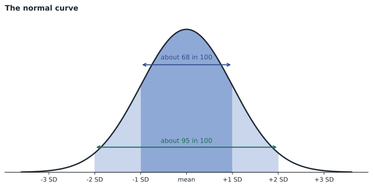
A z-score expresses a score as the number of standard deviations it lies above or below the mean. If an exam has a mean of 70 and a standard deviation of 8, a score of 86 has a z-score of 2, and a score of 62 has a z-score of minus 1. Z-scores allow comparison across different tests: Fatima's z-score of 1.5 in chemistry is more impressive than a z-score of 0.5 in biology, even if her raw biology mark was higher.

Correlation coefficients

Lesson 2 described correlations in words. The correlation coefficient, written r, expresses one as a number from minus 1 to plus 1. The sign shows direction: positive means the variables rise together, negative means one rises as the other falls. The size shows strength: values near zero mean little relationship, and values near plus or minus 1 mean a strong one. A correlation of minus 0.6 is stronger than one of plus 0.3.

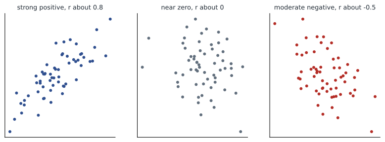
Correlations in psychology are often modest. A correlation of 0.3 between a personality trait and job performance can be useful for prediction across many people while still leaving most individual differences unexplained. Correlations also measure only straight-line relationships; a variable that rises and then falls, like performance as stress increases, can show a correlation near zero even when the relationship is strong.

The class sees another trap when Navarro shows them the illusory correlation: people perceive relationships that are not there, especially when they expect one. Many people believe that more babies are born during full moons or that emergency rooms are busier then. Large studies of birth records and hospital admissions find no such pattern, but the memorable full-moon nights stick in memory while ordinary nights are forgotten.

Is the difference real? Statistical significance

Suppose Navarro randomly assigns half the class to quiz themselves on the reading and half to reread it, and the self-testing group scores 6 points higher on the next exam. Could the difference just be luck? Inferential statistics answer by asking how likely a difference this large would be if the technique had no real effect. That probability is the p-value. By convention, if p is less than 0.05, the result is called statistically significant, meaning a difference this large would occur by chance less than one time in twenty if there were no real effect.

Three things make a result more likely to be significant: a larger difference between groups, less variation within groups and a larger sample. Navarro warns against three common misreadings. A p-value is not the probability that the hypothesis is true. Significant does not mean important; with enormous samples, trivial differences become significant. And a non-significant result does not prove there is no effect; the study may simply have been too small.

Effect sizes and confidence intervals

Because significance depends on sample size, researchers also report effect sizes, which describe how large a difference or relationship is. A common one, Cohen's d, expresses the difference between two group means in standard deviation units.

If the self-testing group scored 6 points higher and the standard deviation of exam scores was 12, then d is 0.5. As a rough guide, Jacob Cohen suggested that 0.2 is a small effect, 0.5 a medium one and 0.8 a large one, although what counts as meaningful depends on the field. A confidence interval gives a range of plausible values for the true effect. A report that self-testing raised scores by 6 points, with a confidence interval at the conventional 95 level running from 2 to 10 points, says much more than 'the result was significant'.

Regression to the mean

One statistical idea explains a surprising number of everyday beliefs. When a score is extreme partly because of chance, the next score from the same person tends to be closer to the average. This is called regression to the mean. A student who scores far above her usual level on one quiz, helped by lucky guesses, will probably score a little lower on the next one, and a student who had an unusually bad day will probably do better next time, whatever anyone does in between.

Regression to the mean fools people because it looks like cause and effect. A coach who shouts at players after an unusually bad game sees them improve in the next game and concludes that shouting works; a coach who praises an unusually good performance sees a decline and concludes that praise makes players lazy. Both are probably watching regression. The same trap affects health claims: people tend to try a new remedy when their symptoms are at their worst, and because symptoms often fluctuate, they are likely to feel better soon afterward whether or not the remedy did anything. Ruth says this explains many of the confident testimonials she heard at the pharmacy counter. The cure is the same as in lesson 2: a comparison group that experiences the same ups and downs without the treatment.

Why sample size matters

Small samples produce more extreme results than large ones, simply because a few unusual individuals have more influence. If a coin is flipped 10 times, getting 8 or more heads is not rare; if it is flipped 1,000 times, getting 800 heads would be astonishing. The same principle applies to studies. A study of 20 people can easily find a large effect by chance, while a study of 2,000 people gives a much more stable estimate. This is one reason the most dramatic findings in psychology have often come from small studies and have often shrunk when tested in larger ones.

The replication crisis

Around 2010, psychologists began to discover that many published findings did not hold up when other researchers repeated them. In 2015, a large collaboration of researchers attempted to replicate 100 studies published in three leading psychology journals. Almost all of the originals had reported significant results, but only about 36 of the replications did, and the average effect in the replications was about half the size of the original. Effects that had become famous, including some claims about willpower being used up like fuel and about brief poses changing hormone levels, proved much weaker or absent when tested again with large samples.

Several practices had contributed. Small samples produce unstable results. Researchers had flexibility in how they analyzed data, such as which outliers to exclude or which measures to report, and trying several analyses until one reaches p less than 0.05, sometimes called p-hacking, produces false positives. Journals preferred surprising, positive results, so failures to find an effect often went unpublished, a problem called publication bias.

Psychology responded with reforms that are now spreading to other sciences. Many researchers preregister their hypotheses, methods and analysis plans before collecting data, so readers can tell planned tests from exploratory ones. Some journals publish registered reports, accepting studies based on their question and design before results are known. Researchers increasingly share their data and materials, use larger samples and run multi-laboratory replications. Navarro tells the class that the crisis is a sign of science working: the field found its own errors and changed its methods. It also means that in this course, a claim is described as established only when it has replicated.