
PHYS-499 · Lesson 8 of 12 · 31 min
Data analysis: fitting, uncertainty and comparing with theory
▶ Video coming soon A video version of this lesson is on the way.
Data analysis is where a project's question is finally answered, and it is where many theses go wrong. The common failures are not arithmetic mistakes but judgments: uncertainties that are calculated but not estimated honestly, comparisons that ignore correlations between errors, fits whose free parameters hide the very discrepancy the project was meant to find, and conclusions that claim more than the data support. This lesson takes Maya's measurements from raw transit times to a comparison with three models. It builds an uncertainty budget, propagates uncertainties analytically and by Monte Carlo, separates errors shared by all pipes from errors that differ between pipes, tests the models with chi-squared, and reports what the data do and do not show. PHYS-397 introduced many of these tools; here they are used to answer a research question.
From raw times to terminal speeds
For each pipe Maya made ten drops, recording the transit time between the gates 0.800 m apart. The mean of the ten times, and its standard error, the sample standard deviation divided by the square root of the number of drops, give the best estimate of the transit time and its statistical uncertainty. The terminal speed is the baseline divided by the mean time. The baseline itself was measured with a steel rule to 0.5 mm, an uncertainty of about 0.06 per 100 that is common to all pipes and negligible compared with the rest.
import math
MU0 = 4e-7*math.pi
G = 9.81

def ellip(k):
    """Complete elliptic integrals K(k) and E(k) by the arithmetic-geometric mean."""
    a, b, c = 1.0, math.sqrt(1 - k*k), k
    tot, n = 0.5*c*c, 0
    while abs(c) > 1e-15:
        a, b, c = (a + b)/2, math.sqrt(a*b), (a - b)/2
        n += 1
        tot += 2**(n - 1)*c*c
    K = math.pi/(2*a)
    return K, K*(1 - tot)

def loop_br(I, R, r, z):
    """Radial field of a circular current loop (radius R, current I) at radius r, height z."""
    q = (R + r)**2 + z*z
    K, E = ellip(math.sqrt(4*R*r/q))
    return MU0*I/(2*math.pi)*z/(r*math.sqrt(q))*(-K + (R*R + r*r + z*z)/((R - r)**2 + z*z)*E)

def dipole_br(m, r, z):
    """Radial field of a point dipole m on the axis."""
    return MU0*m/(4*math.pi)*3*r*z/(r*r + z*z)**2.5

def cylinder_br(m, Rm, Lm, r, z, n=24):
    """Uniformly magnetized cylinder treated as n stacked current loops."""
    M = m/(math.pi*Rm*Rm*Lm); dz = Lm/n
    return sum(loop_br(M*dz, Rm, r, z - (-Lm/2 + (i + 0.5)*dz)) for i in range(n))

def drag_k(br, sigma, a, b, nr=6, zmax=0.10, nz=300):
    """Drag coefficient k = sigma * integral of 2 pi r Br^2 over the wall, so that F = k v."""
    tot, h = 0.0, 2*zmax/nz
    for i in range(nr):
        r = a + (i + 0.5)*(b - a)/nr
        s = sum(br(r, -zmax + (j + 0.5)*h)**2 for j in range(nz))*h
        tot += 2*math.pi*r*sigma*s*(b - a)/nr
    return tot

def k_thin(m, sigma, a, b):
    """Point dipole, thin wall at the mean radius: k = 45 mu0^2 m^2 sigma w / (1024 abar^4)."""
    w, abar = b - a, (a + b)/2
    return 45*MU0**2*m*m*sigma*w/(1024*abar**4)

def k_thick(m, sigma, a, b):
    """Point dipole, wall integrated from a to b exactly."""
    return 45*MU0**2*m*m*sigma*(a**-3 - b**-3)/(3*1024)
# Maya's magnet and pipes (lengths in m)
MASS, RM, LM = 12.10e-3, 6.35e-3, 12.70e-3        # magnet mass (kg), radius, length
PIPES = [  # name, inner radius, outer radius, conductivity (S/m)
    ("Cu M 1/2", 7.228e-3, 7.938e-3, 4.95e7),
    ("Cu L 1/2", 6.918e-3, 7.938e-3, 4.95e7),
    ("Cu K 1/2", 6.698e-3, 7.938e-3, 4.95e7),
    ("Al 1/2",   6.698e-3, 7.938e-3, 2.50e7),
    ("Cu L 3/4", 9.973e-3, 11.113e-3, 4.95e7),
]
import random
def drops(name, n=10, seed=2027):
    """Ten transit times (s) over the 0.800 m between the light gates for one pipe."""
    rnd = random.Random(seed + sum(map(ord, name)))
    true_m = 1.62
    for nm, a, b, sig in PIPES:
        if nm == name: break
    vt = 0.975*MASS*G/drag_k(lambda r, z: cylinder_br(true_m, RM, LM, r, z), sig, a, b)
    return [round(0.800/vt*(1 + rnd.gauss(0, 0.010)) + rnd.gauss(0, 0.001), 3) for _ in range(n)]

import math
print(f"{'pipe':10s} {'mean time (s)':>14s} {'scatter':>8s} {'std error':>10s} {'v_t (cm/s)':>11s} {'rel. unc.':>10s}")
for name, a, b, sig in PIPES:
    t = drops(name); n = len(t); mt = sum(t)/n
    sd = math.sqrt(sum((x - mt)**2 for x in t)/(n - 1)); se = sd/math.sqrt(n)
    v = 0.800/mt
print(f"{name:10s} {mt:14.3f} {sd/mt*100:7.2f}% {se:10.3f} {v*100:11.3f} {se/mt*100:9.2f}%")pipe mean time (s) scatter std error v_t (cm/s) rel. unc. Cu M 1/2 9.636 1.08% 0.033 8.302 0.34% Cu L 1/2 15.039 0.85% 0.041 5.319 0.27% Cu K 1/2 19.689 1.01% 0.063 4.063 0.32% Al 1/2 9.855 1.29% 0.040 8.118 0.41% Cu L 3/4 4.826 0.55% 0.008 16.578 0.18%
The drop-to-drop scatter is about 1 per 100, larger than the 1 ms timing resolution would explain. Maya traced it to small variations in how the magnet tilted and drifted off the axis as it fell, which she could see by marking the magnet and watching through the gate slots. The scatter averages down with repeated drops, so the statistical uncertainty on each mean is about 0.3 per 100. That is smaller than every other uncertainty in the problem, which confirmed that ten drops per pipe was enough. More drops would not have improved the comparison; better knowledge of the inputs would.
Building an uncertainty budget
The prediction of the finite-magnet model depends on the dipole moment, the conductivity, the inner and outer radii, and the mass of the magnet. Each has an uncertainty from its calibration, and each propagates into the predicted speed. When a quantity depends on inputs through a formula \(f(x_1, x_2, \ldots)\), and the input uncertainties are small and independent, the standard propagation rule is
where the logarithmic derivatives are the sensitivities: how many parts per hundred the result changes for each part per hundred change in an input. Some sensitivities follow directly from the physics. The drag is proportional to \(m^2\) and to \(\sigma\), so the speed has sensitivity \(-2\) to the moment and \(-1\) to the conductivity, and \(+1\) to the mass. The sensitivities to the radii have no simple formula for the finite magnet, so Maya computed them numerically by changing each radius by 0.01 mm and recomputing the drag. An uncertainty budget lists each input, its uncertainty, its sensitivity and its contribution, so that a reader can see at a glance what limits the result.
import math
MU0 = 4e-7*math.pi
G = 9.81

def ellip(k):
    """Complete elliptic integrals K(k) and E(k) by the arithmetic-geometric mean."""
    a, b, c = 1.0, math.sqrt(1 - k*k), k
    tot, n = 0.5*c*c, 0
    while abs(c) > 1e-15:
        a, b, c = (a + b)/2, math.sqrt(a*b), (a - b)/2
        n += 1
        tot += 2**(n - 1)*c*c
    K = math.pi/(2*a)
    return K, K*(1 - tot)

def loop_br(I, R, r, z):
    """Radial field of a circular current loop (radius R, current I) at radius r, height z."""
    q = (R + r)**2 + z*z
    K, E = ellip(math.sqrt(4*R*r/q))
    return MU0*I/(2*math.pi)*z/(r*math.sqrt(q))*(-K + (R*R + r*r + z*z)/((R - r)**2 + z*z)*E)

def dipole_br(m, r, z):
    """Radial field of a point dipole m on the axis."""
    return MU0*m/(4*math.pi)*3*r*z/(r*r + z*z)**2.5

def cylinder_br(m, Rm, Lm, r, z, n=24):
    """Uniformly magnetized cylinder treated as n stacked current loops."""
    M = m/(math.pi*Rm*Rm*Lm); dz = Lm/n
    return sum(loop_br(M*dz, Rm, r, z - (-Lm/2 + (i + 0.5)*dz)) for i in range(n))

def drag_k(br, sigma, a, b, nr=6, zmax=0.10, nz=300):
    """Drag coefficient k = sigma * integral of 2 pi r Br^2 over the wall, so that F = k v."""
    tot, h = 0.0, 2*zmax/nz
    for i in range(nr):
        r = a + (i + 0.5)*(b - a)/nr
        s = sum(br(r, -zmax + (j + 0.5)*h)**2 for j in range(nz))*h
        tot += 2*math.pi*r*sigma*s*(b - a)/nr
    return tot

def k_thin(m, sigma, a, b):
    """Point dipole, thin wall at the mean radius: k = 45 mu0^2 m^2 sigma w / (1024 abar^4)."""
    w, abar = b - a, (a + b)/2
    return 45*MU0**2*m*m*sigma*w/(1024*abar**4)

def k_thick(m, sigma, a, b):
    """Point dipole, wall integrated from a to b exactly."""
    return 45*MU0**2*m*m*sigma*(a**-3 - b**-3)/(3*1024)
# Maya's magnet and pipes (lengths in m)
MASS, RM, LM = 12.10e-3, 6.35e-3, 12.70e-3        # magnet mass (kg), radius, length
PIPES = [  # name, inner radius, outer radius, conductivity (S/m)
    ("Cu M 1/2", 7.228e-3, 7.938e-3, 4.95e7),
    ("Cu L 1/2", 6.918e-3, 7.938e-3, 4.95e7),
    ("Cu K 1/2", 6.698e-3, 7.938e-3, 4.95e7),
    ("Al 1/2",   6.698e-3, 7.938e-3, 2.50e7),
    ("Cu L 3/4", 9.973e-3, 11.113e-3, 4.95e7),
]

import math, random
m0 = 1.62
name, a, b, sig = PIPES[1]
def kfin(m, s, a, b): return drag_k(lambda r, z: cylinder_br(m, RM, LM, r, z), s, a, b)
k0 = kfin(m0, sig, a, b); v0 = MASS*G/k0
d = 1e-5                                              # 0.01 mm
dv_da = (MASS*G/kfin(m0, sig, a + d, b) - v0)/v0      # fractional change for +0.01 mm
dv_db = (MASS*G/kfin(m0, sig, a, b + d) - v0)/v0
budget = [  # input, relative uncertainty of input, contribution to v (relative)
    ("dipole moment, 1.62 +/- 0.02 A m^2",   0.02/1.62, 2*0.02/1.62),
    ("conductivity, +/- 1.0 per 100",        0.010,     0.010),
    ("inner radius, +/- 0.01 mm",            d/a,       abs(dv_da)),
    ("outer radius, +/- 0.01 mm",            d/b,       abs(dv_db)),
    ("magnet mass, +/- 0.01 g",              1e-5/MASS, 1e-5/MASS),
    ("numerical integration",                0.0,       4.4e-4),
]
print(f"predicted v_t for {name}: {v0*100:.3f} cm/s")
for what, rin, rout in budget:
    print(f"  {what:38s} contributes {rout*100:5.2f} per 100")
tot = math.sqrt(sum(r*r for _, _, r in budget))
common = math.sqrt(budget[0][2]**2 + budget[1][2]**2)
own = math.sqrt(sum(r*r for _, _, r in budget[2:]))
print(f"  total {tot*100:.2f} per 100: shared by all copper pipes {common*100:.2f}, specific to this pipe {own*100:.2f}")
# Monte Carlo check using the scaling of v with each input
rnd = random.Random(8)
vs = []
for _ in range(20000):
    f = (1 + rnd.gauss(0, budget[0][1]))**-2 * (1 + rnd.gauss(0, 0.010))**-1
    f *= (1 + dv_da*rnd.gauss(0, 1) + dv_db*rnd.gauss(0, 1)) * (1 + rnd.gauss(0, budget[4][1]))
    vs.append(v0*f)
mu = sum(vs)/len(vs); sd = math.sqrt(sum((x - mu)**2 for x in vs)/(len(vs) - 1))
print(f"Monte Carlo: mean {mu*100:.3f} cm/s, standard deviation {sd/mu*100:.2f} per 100")predicted v_t for Cu L 1/2: 5.458 cm/s dipole moment, 1.62 +/- 0.02 A m^2 contributes 2.47 per 100 conductivity, +/- 1.0 per 100 contributes 1.00 per 100 inner radius, +/- 0.01 mm contributes 1.28 per 100 outer radius, +/- 0.01 mm contributes 0.75 per 100 magnet mass, +/- 0.01 g contributes 0.08 per 100 numerical integration contributes 0.04 per 100 total 3.05 per 100: shared by all copper pipes 2.66, specific to this pipe 1.49 Monte Carlo: mean 5.460 cm/s, standard deviation 3.05 per 100
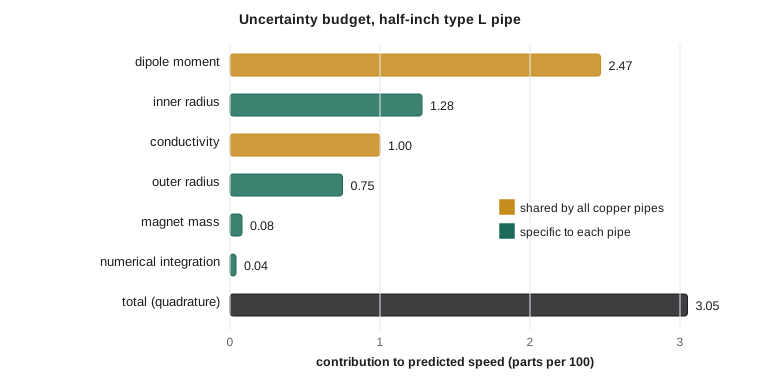
The budget makes two points that shaped the rest of the analysis. First, the dipole moment dominates. Because the drag goes as the square of the moment, its 1.2 per 100 calibration uncertainty becomes about 2.5 per 100 in the prediction, more than the conductivity and both radii together. If Maya had more time, improving the moment calibration would be the most effective way to sharpen the test. Second, the Monte Carlo check, which samples every input from its distribution and recomputes the prediction 20,000 times, agrees with the analytic propagation. That agreement is expected here because the uncertainties are small; when they are large, or when the dependence on an input is strongly nonlinear, the Monte Carlo result is the one to trust.
Shared and independent errors
The budget also separates errors into two kinds, and the distinction is crucial when comparing several measurements with a model. The dipole moment and the copper conductivity are the same for every copper pipe, so if the moment is really 1 per 100 higher than measured, every copper prediction is 2 per 100 too high together. These are correlated, or common, errors. The radii are measured separately for each pipe, so their errors are independent. Statistical errors in the timing are independent too. Treating correlated errors as independent is one of the most common mistakes in data analysis, because it makes a set of measurements look more inconsistent with a model than it is, or more consistent, depending on the pattern.
The clean way to handle this is to split the comparison in two. First test the shape: are the ratios of measured to predicted speed consistent with one another across the pipes, using only the independent uncertainties? A model that fails this test is wrong in its dependence on radius, thickness or material, and no adjustment of the moment or conductivity can rescue it. Then test the scale: is the common ratio consistent with 1, given the shared uncertainty? A model that passes the shape test but fails the scale test may be right in its physics but wrong in an input, or may be missing a small effect that acts the same way in every pipe.
Comparing three models with the data
import math
MU0 = 4e-7*math.pi
G = 9.81

def ellip(k):
    """Complete elliptic integrals K(k) and E(k) by the arithmetic-geometric mean."""
    a, b, c = 1.0, math.sqrt(1 - k*k), k
    tot, n = 0.5*c*c, 0
    while abs(c) > 1e-15:
        a, b, c = (a + b)/2, math.sqrt(a*b), (a - b)/2
        n += 1
        tot += 2**(n - 1)*c*c
    K = math.pi/(2*a)
    return K, K*(1 - tot)

def loop_br(I, R, r, z):
    """Radial field of a circular current loop (radius R, current I) at radius r, height z."""
    q = (R + r)**2 + z*z
    K, E = ellip(math.sqrt(4*R*r/q))
    return MU0*I/(2*math.pi)*z/(r*math.sqrt(q))*(-K + (R*R + r*r + z*z)/((R - r)**2 + z*z)*E)

def dipole_br(m, r, z):
    """Radial field of a point dipole m on the axis."""
    return MU0*m/(4*math.pi)*3*r*z/(r*r + z*z)**2.5

def cylinder_br(m, Rm, Lm, r, z, n=24):
    """Uniformly magnetized cylinder treated as n stacked current loops."""
    M = m/(math.pi*Rm*Rm*Lm); dz = Lm/n
    return sum(loop_br(M*dz, Rm, r, z - (-Lm/2 + (i + 0.5)*dz)) for i in range(n))

def drag_k(br, sigma, a, b, nr=6, zmax=0.10, nz=300):
    """Drag coefficient k = sigma * integral of 2 pi r Br^2 over the wall, so that F = k v."""
    tot, h = 0.0, 2*zmax/nz
    for i in range(nr):
        r = a + (i + 0.5)*(b - a)/nr
        s = sum(br(r, -zmax + (j + 0.5)*h)**2 for j in range(nz))*h
        tot += 2*math.pi*r*sigma*s*(b - a)/nr
    return tot

def k_thin(m, sigma, a, b):
    """Point dipole, thin wall at the mean radius: k = 45 mu0^2 m^2 sigma w / (1024 abar^4)."""
    w, abar = b - a, (a + b)/2
    return 45*MU0**2*m*m*sigma*w/(1024*abar**4)

def k_thick(m, sigma, a, b):
    """Point dipole, wall integrated from a to b exactly."""
    return 45*MU0**2*m*m*sigma*(a**-3 - b**-3)/(3*1024)
# Maya's magnet and pipes (lengths in m)
MASS, RM, LM = 12.10e-3, 6.35e-3, 12.70e-3        # magnet mass (kg), radius, length
PIPES = [  # name, inner radius, outer radius, conductivity (S/m)
    ("Cu M 1/2", 7.228e-3, 7.938e-3, 4.95e7),
    ("Cu L 1/2", 6.918e-3, 7.938e-3, 4.95e7),
    ("Cu K 1/2", 6.698e-3, 7.938e-3, 4.95e7),
    ("Al 1/2",   6.698e-3, 7.938e-3, 2.50e7),
    ("Cu L 3/4", 9.973e-3, 11.113e-3, 4.95e7),
]
import random
def drops(name, n=10, seed=2027):
    """Ten transit times (s) over the 0.800 m between the light gates for one pipe."""
    rnd = random.Random(seed + sum(map(ord, name)))
    true_m = 1.62
    for nm, a, b, sig in PIPES:
        if nm == name: break
    vt = 0.975*MASS*G/drag_k(lambda r, z: cylinder_br(true_m, RM, LM, r, z), sig, a, b)
    return [round(0.800/vt*(1 + rnd.gauss(0, 0.010)) + rnd.gauss(0, 0.001), 3) for _ in range(n)]

import math
m0 = 1.62
def kfin(m, s, a, b): return drag_k(lambda r, z: cylinder_br(m, RM, LM, r, z), s, a, b)
rows = []
for name, a, b, sig in PIPES:
    t = drops(name); n = len(t); mt = sum(t)/n
    se = math.sqrt(sum((x - mt)**2 for x in t)/(n - 1)/n)
    v = 0.800/mt
    d = 1e-5; k0 = kfin(m0, sig, a, b)
    geo = math.hypot(kfin(m0, sig, a + d, b)/k0 - 1, kfin(m0, sig, a, b + d)/k0 - 1)
    own = math.hypot(geo, se/mt)                       # independent part, relative
    preds = {"thin dipole": MASS*G/k_thin(m0, sig, a, b), "thick dipole": MASS*G/k_thick(m0, sig, a, b),
             "finite magnet": MASS*G/k0}
    rows.append((name, v, own, preds))
common = math.hypot(2*0.02/1.62, 0.010)
print(f"independent uncertainty per pipe {min(r[2] for r in rows)*100:.1f} to {max(r[2] for r in rows)*100:.1f} per 100; shared {common*100:.1f} per 100")
for model in ["thin dipole", "thick dipole", "finite magnet"]:
    ratios = [(v/p[model], u) for _, v, u, p in rows]
    w = [1/u**2 for _, u in ratios]
    s = sum(wi*r for wi, (r, _) in zip(w, ratios))/sum(w)          # weighted mean ratio
    chi2 = sum(((r - s)/u)**2 for r, u in ratios)
    print(f"{model:13s} measured/predicted: " + " ".join(f"{r:.3f}" for r, _ in ratios))
    print(f"{'':13s} shape test: chi-squared {chi2:6.1f} for {len(ratios) - 1} degrees of freedom;"
          f" scale {s:.3f}, which is {(s - 1)/common:+.1f} shared standard uncertainties from 1")
cu_k = [r for r in rows if r[0] == "Cu K 1/2"][0]; al = [r for r in rows if r[0] == "Al 1/2"][0]
print(f"H1, same geometry: speed ratio Al/Cu = {al[1]/cu_k[1]:.3f}, conductivity ratio {4.95/2.50:.3f}")independent uncertainty per pipe 1.3 to 2.1 per 100; shared 2.7 per 100
thin dipole measured/predicted: 1.354 1.354 1.334 1.346 1.162
shape test: chi-squared 152.9 for 4 degrees of freedom; scale 1.300, which is +11.3 shared standard uncertainties from 1
thick dipole measured/predicted: 1.364 1.375 1.367 1.379 1.173
shape test: chi-squared 179.1 for 4 degrees of freedom; scale 1.323, which is +12.1 shared standard uncertainties from 1
finite magnet measured/predicted: 0.974 0.975 0.968 0.977 0.974
shape test: chi-squared 0.2 for 4 degrees of freedom; scale 0.973, which is -1.0 shared standard uncertainties from 1
H1, same geometry: speed ratio Al/Cu = 1.998, conductivity ratio 1.980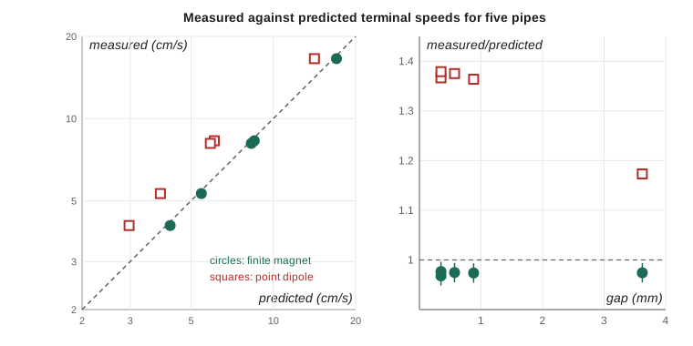
The results are unambiguous about the point-dipole models. Both fail the shape test with a chi-squared of 150 to 180 for four degrees of freedom: the measured speeds exceed the predictions by about 37 per 100 in the half-inch pipes but only about 17 per 100 in the three-quarter-inch pipe. The failure depends on the gap between magnet and wall, exactly as the finite-magnet analysis predicted, so it cannot be blamed on a wrong moment or conductivity, which would shift every pipe by the same factor. H2 is rejected. The finite-magnet model passes the shape test comfortably, with a chi-squared of 0.2 for four degrees of freedom, well below the expected value of about 4, which suggests that the independent uncertainties, dominated by the radii, are if anything a little conservative. Its common ratio is about 0.973: the magnet falls about 2.7 per 100 more slowly than predicted in every pipe. That is about one shared standard uncertainty from perfect agreement, so the data are consistent with H3. H1 holds too: the speed ratio between the aluminum and copper pipes of identical size matches the conductivity ratio within the uncertainties.
Interpreting a small residual
A one-standard-deviation residual is not evidence of new physics, but it is worth asking whether it has a cause. Maya listed candidates and tested what she could. If the moment were 1.3 per 100 higher than her calibration, the residual would vanish, but that is just inside her calibration uncertainty and she had no independent reason to think it was. If the magnet drifts off the axis, the drag rises, because the side nearer the wall sees a stronger field; a numerical estimate showed that an average offset of about 0.15 mm would slow the magnet by roughly 2 per 100, and her observations through the gate slots suggested offsets of that size. Friction with the wall, which the steel slug control ruled out for a nonmagnetic object, could still occur when an off-axis magnet is attracted to its own image currents. She concluded that the finite-magnet model accounts for the data within its stated uncertainty, that off-axis motion is the most plausible source of the small remaining slowdown, and that a tighter test would need a better moment calibration and a way to keep the magnet centered.
Consider what she did not do. She did not add a fitted correction factor to the model and then claim agreement; she reported the parameter-free comparison first, then quantified the residual. She did not drop the pipe with the largest residual. She did not describe a one-sigma effect as a discovery. And she reported the failure of the point-dipole model as a clear result in its own right, because showing exactly how and why a widely used formula fails is valuable. A thesis that presents its comparison this way gives the examiner every reason to trust its conclusions.
Fitting with care
Fitting is often the right tool, but every free parameter is a choice that needs justification. When Maya fitted the common scale factor, she reported it as a measured quantity with its uncertainty, about \(0.973 \pm 0.007\) from the independent errors alone, and compared it with the shared uncertainty of the prediction, about 2.7 per 100. She also checked that the fit was not hiding anything: the chi-squared after the fit was small, and the residuals showed no trend with the gap, the wall thickness or the metal. A fit with too many free parameters can match almost anything; the more parameters a model needs, the less a good fit tells you. The strongest evidence a thesis can offer is a parameter-free prediction that agrees with independent measurements, and the next strongest is a fit whose few parameters have physical meaning and agree with independent determinations.
Worked problem
Reading a chi-squared
A model compared with five pipes gives a chi-squared of 3.1 for 4 degrees of freedom. Another gives 179 for 4. What can you conclude?
Show solution
- For 4 degrees of freedom the expected chi-squared is about 4, with a typical spread of \(\sqrt{2 \times 4} \approx 2.8\).
- A value of 3.1 is entirely typical: the model's predictions are consistent with one another within the stated uncertainties. The probability of a value at least this large, if the model is right, is about 0.54.
- A value of 179 is impossible by chance: the model is wrong in its dependence on the pipe parameters, or the uncertainties are badly underestimated.
- Since the second model is the point dipole and the residuals follow the gap to the wall, the model is wrong, not the uncertainties.
Answer: The first model is consistent with the data; the second is decisively rejected.
Common mistakes
MistakeTreating shared errors, such as the dipole moment, as independent for each pipe.
InsteadSeparate the comparison into a shape test with independent errors and a scale test with shared errors.
MistakeQuoting only the statistical uncertainty.
InsteadBuild a full budget of every input; here the statistical part was the smallest.
MistakeAdding a fitted factor and then claiming the model agrees.
InsteadReport the parameter-free comparison first, then quantify any residual.
MistakeCalling a one-standard-deviation residual a discovery, or ignoring it.
InsteadReport it, list possible causes, test what you can, and state what a sharper test would need.
MistakeDropping the point that disagrees most.
InsteadKeep all data unless there is a documented, independent reason to exclude a point.
Summary and key terms
- Compute means, standard errors and terminal speeds from repeated drops; here the statistical uncertainty was about 0.3 per 100, the smallest in the budget.
- Propagate input uncertainties with logarithmic sensitivities and check with Monte Carlo; the dipole moment dominated through the square in the drag.
- Separate shared errors from independent ones: test the shape of a model against several measurements with independent errors, then the scale with shared errors.
- The point-dipole models failed the shape test decisively, with errors that grew as the gap to the wall shrank; the finite-magnet model passed, with a common ratio of 0.973, one shared standard uncertainty from 1.
- Report parameter-free comparisons first, treat small residuals honestly, and justify every fitted parameter.
- Standard error
- The standard deviation of the mean: the sample standard deviation divided by the square root of the number of measurements.
- Sensitivity
- The fractional change in a result per fractional change in an input.
- Uncertainty budget
- A table of every input uncertainty and its contribution to the final uncertainty.
- Correlated error
- An error shared by several measurements, so they move together.
- Chi-squared
- The sum of squared residuals in units of their uncertainties, used to test a model.
Practice problems
Work each problem on paper first, then reveal the answer to check.
If the dipole moment were 1.2 per 100 higher than measured, how would every finite-magnet prediction change?
Show answer
The drag rises by 2.4 per 100, so every predicted speed falls by about 2.4 per 100, and the common ratio rises from 0.973 to about 0.997.
Why can a wrong conductivity not explain the point-dipole failure?
Show answer
A wrong conductivity would shift all copper pipes by the same factor, but the point-dipole errors differ between pipes and follow the gap.
Ten drops gave a scatter of 1 per 100. How many drops would halve the statistical uncertainty, and would it help?
Show answer
Forty drops; it would not help much, since the statistical part is already far below the moment and radius contributions.
In the budget, why is the inner radius more important than the outer radius?
Show answer
The inner surface is closer to the magnet, where the radial field is strongest, so the drag is more sensitive to its position.
What is the probability meaning of a chi-squared equal to the degrees of freedom?
Show answer
It is a typical value if the model is right and the uncertainties are correct; the probability of exceeding it is a little under one half.
Lesson quiz · 5 questions
Score 60% or more to complete this lesson.
Create a free account to save your progress, take quizzes and earn a certificate.