Computational research: models, validation and reproducible code

Almost every physics thesis now involves code, whether to simulate a system, to fit data or to compute a prediction that no closed-form formula provides. Code makes research possible that would otherwise be out of reach, but it also introduces a new kind of error: a program can run without complaint and produce a beautiful, wrong answer. The discipline of computational research is therefore less about writing code than about establishing that the code is right. This lesson builds Maya's model of the eddy-current drag from Faraday's law, derives the point-dipole result that her code must reproduce, validates the numerical model against it, and sets out the habits that make computational work reproducible.

Deriving the drag on a falling dipole

Work in the frame of the magnet, so that the pipe moves upward past it at speed \(v\). Consider a thin ring of the pipe wall at radius \(r\), height \(z\) above the magnet's center, with axial thickness \(dz\) and radial thickness \(dr\). The magnet's field at the ring has an axial component \(B_z\) and a radial component \(B_r\). As the ring moves with velocity \(v\hat{z}\) through the field, each charge in it feels a magnetic force \(q\,\mathbf{v} \times \mathbf{B}\). Only the radial component of the field contributes an azimuthal force, so there is an azimuthal electric field, in effect, of size \(v B_r\) around the ring. The resulting electromotive force around the ring is

The same result follows from Faraday's law, since the rate at which the flux through the moving ring changes is \(v\,\partial\Phi/\partial z\), and the flux gradient is related to the radial field by the absence of magnetic monopoles. The ring has resistance \(dR = 2\pi r/(\sigma\, dz\, dr)\), so the current in it is \(dI = \mathcal{E}/dR = \sigma v B_r\, dz\, dr\). This assumes the induced currents are small enough that their own magnetic field does not appreciably change \(B_r\), which holds when the speed is low; the condition, examined in the thesis, is that the magnetic Reynolds number \(\mu_0 \sigma v w\) is much less than one, and for Maya's speeds of a few centimeters per second it is about \(10^{-3}\).

The force on the ring follows from \(dI\,d\mathbf{l} \times \mathbf{B}\). Again only \(B_r\) matters for the axial force, and integrating around the ring gives an axial force of size \(2\pi r\, dI\, B_r = 2\pi r \sigma v B_r^2\, dz\, dr\). By Newton's third law the magnet feels the opposite force, which opposes its motion relative to the pipe. Adding the contributions of all rings gives a drag \(F = k v\) with

This expression is general: it holds for any axially symmetric magnet whose field is known, which is why Maya's code computes exactly this double integral. It also makes a useful physical point visible. The drag depends on the square of the radial field, integrated over the wall, so it is dominated by the parts of the wall closest to the magnet's poles, where the field lines bend outward most strongly. A model that gets the field near the wall wrong will get the drag wrong, which is exactly the weakness of the point-dipole approximation for a magnet that nearly fills the pipe.

For a point dipole of moment \(m\) on the axis, the radial field is \(B_r = (\mu_0 m/4\pi)\,3 r z/(r^2 + z^2)^{5/2}\). Substituting and using the integral

the inner integral over \(z\) gives \(2\pi r\,(\mu_0 m/4\pi)^2\, 9 r^2 \cdot 5\pi/(128 r^7) = 45 \mu_0^2 m^2/(1024\, r^4)\). For a thin wall of thickness \(w\) at radius \(a\), multiplying by \(\sigma w\) gives the textbook result \(k = 45 \mu_0^2 m^2 \sigma w/(1024 a^4)\), which explains the curious factor of 45/1024. For a thick wall, the radial integral can be done exactly:

Deriving these formulas was the third pass on Maya's key paper, and it gave her more than a check on the algebra. It gave her two exact results that her numerical code must reproduce: the thin-wall formula in the limit of small wall thickness, and the thick-wall formula for any thickness, both for a point dipole. Exact special cases like these are the most valuable tools in validating any numerical model.

The finite-magnet model

A real cylindrical magnet is not a point. A uniformly magnetized cylinder has the same field as a sheet of azimuthal current on its curved surface with current per unit length equal to the magnetization \(M = m/(\pi R^2 L)\), so it can be represented exactly as a stack of thin current loops of radius \(R\). The radial field of a single loop at any point is known in closed form in terms of the complete elliptic integrals \(K\) and \(E\), which can be computed rapidly and to full precision by the arithmetic-geometric mean, the same algorithm PHYS-244 used for the large-amplitude pendulum. Maya's model adds the radial fields of 24 loops and integrates the square over the wall with the midpoint rule. Close to the magnet the finite cylinder's field is weaker and less sharply peaked than a point dipole's, because the moment is spread over a length comparable to the gap between the magnet and the wall. Since the drag depends on the square of the field near the wall, the finite model predicts noticeably less drag.

Validating the code

Validation means showing, with evidence, that the code computes what it is supposed to compute. The standard tools are exact special cases, convergence tests, limiting cases, conservation laws and comparison with independent methods. Maya used the first three. For the point-dipole field, her numerical integral must reproduce the exact thick-wall formula. As the integration grid is refined, the result must converge, and it must not depend on the cutoff of the integral in \(z\). And as the pipe radius grows large compared with the magnet, the finite-magnet result must approach the point-dipole result, because far from the magnet its field is a dipole field.

import math
MU0 = 4e-7*math.pi
G = 9.81

def ellip(k):
    """Complete elliptic integrals K(k) and E(k) by the arithmetic-geometric mean."""
    a, b, c = 1.0, math.sqrt(1 - k*k), k
    tot, n = 0.5*c*c, 0
    while abs(c) > 1e-15:
        a, b, c = (a + b)/2, math.sqrt(a*b), (a - b)/2
        n += 1
        tot += 2**(n - 1)*c*c
    K = math.pi/(2*a)
    return K, K*(1 - tot)

def loop_br(I, R, r, z):
    """Radial field of a circular current loop (radius R, current I) at radius r, height z."""
    q = (R + r)**2 + z*z
    K, E = ellip(math.sqrt(4*R*r/q))
    return MU0*I/(2*math.pi)*z/(r*math.sqrt(q))*(-K + (R*R + r*r + z*z)/((R - r)**2 + z*z)*E)

def dipole_br(m, r, z):
    """Radial field of a point dipole m on the axis."""
    return MU0*m/(4*math.pi)*3*r*z/(r*r + z*z)**2.5

def cylinder_br(m, Rm, Lm, r, z, n=24):
    """Uniformly magnetized cylinder treated as n stacked current loops."""
    M = m/(math.pi*Rm*Rm*Lm); dz = Lm/n
    return sum(loop_br(M*dz, Rm, r, z - (-Lm/2 + (i + 0.5)*dz)) for i in range(n))

def drag_k(br, sigma, a, b, nr=6, zmax=0.10, nz=300):
    """Drag coefficient k = sigma * integral of 2 pi r Br^2 over the wall, so that F = k v."""
    tot, h = 0.0, 2*zmax/nz
    for i in range(nr):
        r = a + (i + 0.5)*(b - a)/nr
        s = sum(br(r, -zmax + (j + 0.5)*h)**2 for j in range(nz))*h
        tot += 2*math.pi*r*sigma*s*(b - a)/nr
    return tot

def k_thin(m, sigma, a, b):
    """Point dipole, thin wall at the mean radius: k = 45 mu0^2 m^2 sigma w / (1024 abar^4)."""
    w, abar = b - a, (a + b)/2
    return 45*MU0**2*m*m*sigma*w/(1024*abar**4)

def k_thick(m, sigma, a, b):
    """Point dipole, wall integrated from a to b exactly."""
    return 45*MU0**2*m*m*sigma*(a**-3 - b**-3)/(3*1024)
# Maya's magnet and pipes (lengths in m)
MASS, RM, LM = 12.10e-3, 6.35e-3, 12.70e-3        # magnet mass (kg), radius, length
PIPES = [  # name, inner radius, outer radius, conductivity (S/m)
    ("Cu M 1/2", 7.228e-3, 7.938e-3, 4.95e7),
    ("Cu L 1/2", 6.918e-3, 7.938e-3, 4.95e7),
    ("Cu K 1/2", 6.698e-3, 7.938e-3, 4.95e7),
    ("Al 1/2",   6.698e-3, 7.938e-3, 2.50e7),
    ("Cu L 3/4", 9.973e-3, 11.113e-3, 4.95e7),
]

m = 1.62
name, a, b, sig = PIPES[1]
exact = k_thick(m, sig, a, b)
print(f"point dipole, {name}: exact thick-wall k = {exact:.5f} kg/s")
for nr, nz, zmax in [(2, 100, 0.05), (4, 200, 0.10), (6, 300, 0.10), (12, 600, 0.20)]:
    num = drag_k(lambda r, z: dipole_br(m, r, z), sig, a, b, nr, zmax, nz)
    print(f"  grid nr={nr:2d} nz={nz:3d} zmax={zmax:.2f} m: k = {num:.5f}  relative error {num/exact - 1:+.1e}")
print("thin-wall formula at mean radius:", f"{k_thin(m, sig, a, b):.5f}", "(differs from thick-wall by",
      f"{k_thin(m, sig, a, b)/exact - 1:+.3f})")
print("finite magnet approaches the dipole in wide pipes (ratio k_cylinder / k_dipole):")
for a2 in [0.008, 0.012, 0.020, 0.040]:
    b2 = a2 + 1.0e-3
    kc = drag_k(lambda r, z: cylinder_br(m, RM, LM, r, z), sig, a2, b2, 4, 0.25, 500)
    kd = k_thick(m, sig, a2, b2)
    print(f"  inner radius {a2*1e3:4.0f} mm: {kc/kd:.4f}")

point dipole, Cu L 1/2: exact thick-wall k = 3.06845 kg/s
  grid nr= 2 nz=100 zmax=0.05 m: k = 3.05624  relative error -4.0e-03
  grid nr= 4 nz=200 zmax=0.10 m: k = 3.06538  relative error -1.0e-03
  grid nr= 6 nz=300 zmax=0.10 m: k = 3.06708  relative error -4.4e-04
  grid nr=12 nz=600 zmax=0.20 m: k = 3.06810  relative error -1.1e-04
thin-wall formula at mean radius: 3.02051 (differs from thick-wall by -0.016)
finite magnet approaches the dipole in wide pipes (ratio k_cylinder / k_dipole):
  inner radius    8 mm: 0.7512
  inner radius   12 mm: 0.8816
  inner radius   20 mm: 0.9605
  inner radius   40 mm: 0.9907

The checks pass. At the production grid the numerical integral matches the exact formula to about 4 parts in ten thousand, far below the other uncertainties, and the error falls by roughly a factor of four each time the grid is refined, which shows that the midpoint rule is converging as expected rather than agreeing by accident. The thin-wall formula at the mean radius is within about 2 per 100 of the exact thick-wall result for this pipe, so the thin-wall approximation itself is not the main problem. The finite-magnet ratio rises toward 1 as the pipe widens, reaching about 0.99 at 40 mm, exactly the limiting behavior expected. Together these tests make a convincing case that the code computes the integral correctly. They do not show that the integral is the right physics; only comparison with measurements can do that.

The distinction between those two questions is important enough to have names. Verification asks whether the code solves the equations correctly. Validation, in the stricter sense used in engineering and computational science, asks whether the equations describe reality. Exact special cases and convergence tests verify; comparison with experiment validates. A thesis should report both, and should be clear about which is which.

The predictions

With the code verified, Maya computed the predicted terminal speed for each pipe from the three models: the thin-wall point dipole, the thick-wall point dipole and the thick-wall finite magnet. All used her measured moment, conductivities and dimensions, with no adjustable parameters. She committed these predictions, with their uncertainties from lesson 8, to her repository before analyzing the main data set, which is a simple and effective way of documenting that the predictions were not tuned to the results.

import math
MU0 = 4e-7*math.pi
G = 9.81

def ellip(k):
    """Complete elliptic integrals K(k) and E(k) by the arithmetic-geometric mean."""
    a, b, c = 1.0, math.sqrt(1 - k*k), k
    tot, n = 0.5*c*c, 0
    while abs(c) > 1e-15:
        a, b, c = (a + b)/2, math.sqrt(a*b), (a - b)/2
        n += 1
        tot += 2**(n - 1)*c*c
    K = math.pi/(2*a)
    return K, K*(1 - tot)

def loop_br(I, R, r, z):
    """Radial field of a circular current loop (radius R, current I) at radius r, height z."""
    q = (R + r)**2 + z*z
    K, E = ellip(math.sqrt(4*R*r/q))
    return MU0*I/(2*math.pi)*z/(r*math.sqrt(q))*(-K + (R*R + r*r + z*z)/((R - r)**2 + z*z)*E)

def dipole_br(m, r, z):
    """Radial field of a point dipole m on the axis."""
    return MU0*m/(4*math.pi)*3*r*z/(r*r + z*z)**2.5

def cylinder_br(m, Rm, Lm, r, z, n=24):
    """Uniformly magnetized cylinder treated as n stacked current loops."""
    M = m/(math.pi*Rm*Rm*Lm); dz = Lm/n
    return sum(loop_br(M*dz, Rm, r, z - (-Lm/2 + (i + 0.5)*dz)) for i in range(n))

def drag_k(br, sigma, a, b, nr=6, zmax=0.10, nz=300):
    """Drag coefficient k = sigma * integral of 2 pi r Br^2 over the wall, so that F = k v."""
    tot, h = 0.0, 2*zmax/nz
    for i in range(nr):
        r = a + (i + 0.5)*(b - a)/nr
        s = sum(br(r, -zmax + (j + 0.5)*h)**2 for j in range(nz))*h
        tot += 2*math.pi*r*sigma*s*(b - a)/nr
    return tot

def k_thin(m, sigma, a, b):
    """Point dipole, thin wall at the mean radius: k = 45 mu0^2 m^2 sigma w / (1024 abar^4)."""
    w, abar = b - a, (a + b)/2
    return 45*MU0**2*m*m*sigma*w/(1024*abar**4)

def k_thick(m, sigma, a, b):
    """Point dipole, wall integrated from a to b exactly."""
    return 45*MU0**2*m*m*sigma*(a**-3 - b**-3)/(3*1024)
# Maya's magnet and pipes (lengths in m)
MASS, RM, LM = 12.10e-3, 6.35e-3, 12.70e-3        # magnet mass (kg), radius, length
PIPES = [  # name, inner radius, outer radius, conductivity (S/m)
    ("Cu M 1/2", 7.228e-3, 7.938e-3, 4.95e7),
    ("Cu L 1/2", 6.918e-3, 7.938e-3, 4.95e7),
    ("Cu K 1/2", 6.698e-3, 7.938e-3, 4.95e7),
    ("Al 1/2",   6.698e-3, 7.938e-3, 2.50e7),
    ("Cu L 3/4", 9.973e-3, 11.113e-3, 4.95e7),
]

m = 1.62
print(f"{'pipe':10s} {'thin dipole':>12s} {'thick dipole':>13s} {'finite magnet':>14s}   (terminal speed, cm/s)")
for name, a, b, sig in PIPES:
    v = [MASS*G/k for k in (k_thin(m, sig, a, b), k_thick(m, sig, a, b),
                            drag_k(lambda r, z: cylinder_br(m, RM, LM, r, z), sig, a, b))]
    gap = (a - RM)*1e3
    print(f"{name:10s} {v[0]*100:12.3f} {v[1]*100:13.3f} {v[2]*100:14.3f}   gap to wall {gap:.2f} mm, ratio {v[2]/v[1]:.3f}")

pipe        thin dipole  thick dipole  finite magnet   (terminal speed, cm/s)
Cu M 1/2          6.132         6.087          8.527   gap to wall 0.88 mm, ratio 1.401
Cu L 1/2          3.930         3.868          5.458   gap to wall 0.57 mm, ratio 1.411
Cu K 1/2          3.045         2.973          4.198   gap to wall 0.35 mm, ratio 1.412
Al 1/2            6.030         5.887          8.312   gap to wall 0.35 mm, ratio 1.412
Cu L 3/4         14.270        14.132         17.019   gap to wall 3.62 mm, ratio 1.204

The predictions differ a lot. For the tight half-inch pipes the finite-magnet model predicts speeds about 40 per 100 higher than the point-dipole models, and the difference shrinks for the three-quarter-inch pipe, where the gap between the magnet and the wall is larger. That pattern is itself a prediction: if the finite-magnet model is right, the failure of the point-dipole model should depend on the gap. Lesson 8 compares all three with the data.

Simulating the fall

The predictions assume that the magnet moves at its terminal speed throughout the timed section. That is easy to check by solving the equation of motion \(M\,dv/dt = Mg - kv\), whose exact solution is \(v(t) = v_t(1 - e^{-t/\tau})\) with \(\tau = v_t/g\). A short numerical integration, checked against the exact solution, confirms that the speed is constant to better than one part in a million by the time the magnet reaches the first gate, and also lets Maya ask what happens if the magnet enters with some speed of its own, for example if it is released from slightly above the pipe.

import math
M, g = 12.10e-3, 9.81
k = 2.18                                   # kg/s, finite-magnet value for the half-inch type L pipe
vt, tau = M*g/k, M*g/k/g
def simulate(v0, dt=1e-5, z_gate=0.100):
    t, z, v = 0.0, 0.0, v0
    while z < z_gate:                      # RK4 for dv/dt = g - (k/M) v
        f = lambda u: g - k/M*u
        k1 = f(v); k2 = f(v + dt*k1/2); k3 = f(v + dt*k2/2); k4 = f(v + dt*k3)
        z += dt*(v + dt*(k1 + 2*k2 + 2*k3)/6/2)
        v += dt*(k1 + 2*k2 + 2*k3 + k4)/6; t += dt
    return t, v
print(f"terminal speed {vt*100:.3f} cm/s, time constant {tau*1e3:.2f} ms")
for v0 in [0.0, 0.5, 2.0]:
    t, v = simulate(v0)
    print(f"entry speed {v0:.1f} m/s: at the first gate after {t:.2f} s, v/vt - 1 = {v/vt - 1:+.1e}")
t = 5*tau
print(f"check against exact solution at t = 5 tau: {vt*(1 - math.exp(-5)):.6f} m/s")

terminal speed 5.445 cm/s, time constant 5.55 ms
entry speed 0.0 m/s: at the first gate after 1.84 s, v/vt - 1 = -3.5e-14
entry speed 0.5 m/s: at the first gate after 1.79 s, v/vt - 1 = +3.5e-14
entry speed 2.0 m/s: at the first gate after 1.64 s, v/vt - 1 = +3.5e-14
check against exact solution at t = 5 tau: 0.054083 m/s

Reproducible code

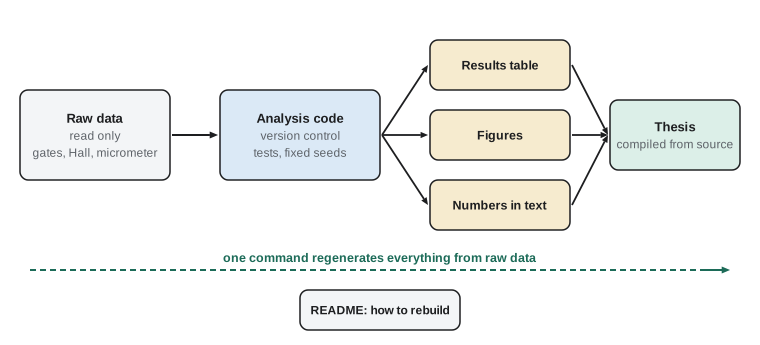
A computational result is reproducible if someone else, or you in six months, can run the same code on the same inputs and get the same answer. That sounds trivial and is often not true, because results depend on code versions, library versions, random seeds, hidden settings and files that were edited by hand. The habits that make code reproducible are straightforward. Keep all code under version control, with Git as the standard tool, committing small changes with clear messages. Never edit data files by hand; keep raw data read-only and do every transformation in code. Fix random seeds and record them. Record the versions of the language and any libraries. Write a short README that explains how to go from raw data to every figure and number in the thesis with one or two commands. And test the code automatically, so that the validation checks above run every time the code changes.

import hashlib, json, random
def analysis(seed=2027):
    rnd = random.Random(seed)
    times = [15.0*(1 + rnd.gauss(0, 0.01)) for _ in range(10)]
    mean = sum(times)/len(times)
    return {"mean_time_s": round(mean, 4), "speed_cm_s": round(80/mean, 4)}
def fingerprint(result):
    return hashlib.sha256(json.dumps(result, sort_keys=True).encode()).hexdigest()[:16]
r1, r2, r3 = analysis(), analysis(), analysis(seed=2028)
print("run 1:", r1, fingerprint(r1))
print("run 2:", r2, fingerprint(r2))
print("same seed reproduces exactly:", fingerprint(r1) == fingerprint(r2))
print("different seed:", r3, fingerprint(r3))

run 1: {'mean_time_s': 15.0247, 'speed_cm_s': 5.3246} 0dbdb70f6b98e948
run 2: {'mean_time_s': 15.0247, 'speed_cm_s': 5.3246} 0dbdb70f6b98e948
same seed reproduces exactly: True
different seed: {'mean_time_s': 15.0618, 'speed_cm_s': 5.3115} 73597013010ebb15

Fingerprinting results, as in the last example, is a cheap way to detect when something has changed. Maya stored a fingerprint of her final results table in the repository; any later change to code, data or library that altered a number would change the fingerprint and be noticed. Jae-won, whose matched-filter search used published noise curves and template banks, went further and recorded the exact version of every public data file he downloaded, because the LIGO open data releases are occasionally updated. Neither habit takes more than a few minutes, and both make it far easier to answer the examiner's question that every computational thesis eventually meets: how do you know this number is right?