Laser principles: threshold, rate equations and output power

We now have the two halves of a laser: a gain medium that amplifies light (lessons 2 and 3) and a resonator that feeds light back and selects modes (lesson 4). This lesson puts them together. We derive the threshold condition, the gain needed for oscillation to start; write the rate equations that couple the population inversion to the number of photons in the cavity; solve them for the steady-state output power; and then follow a laser as it switches on, showing the spikes and relaxation oscillations that appear before it settles. The lesson ends with the slope efficiency, the quantity an engineer most wants to know about a laser.

The threshold condition

Consider a gain medium of length \(\ell\) inside a cavity with mirror reflectivities \(R_1\) and \(R_2\). Besides the mirror transmission, light suffers internal losses from scattering, absorption by impurities and diffraction at apertures, which we lump into a loss coefficient \(\alpha\) per unit length. A wave that makes one round trip has its intensity multiplied by

If this factor is less than one, any light in the cavity dies away. If it exceeds one, a small seed of spontaneous emission grows exponentially. The threshold is where it equals one:

The threshold gain coefficient equals the internal loss plus the mirror loss averaged over the length of the medium. Using \(\gamma = \sigma\Delta N\), the threshold inversion is \(\Delta N_{th} = \gamma_{th}/\sigma\). An equivalent way to write the threshold uses the photon lifetime of lesson 4. If light travels at speed \(c/n\) in the medium and the cavity is filled by it, the gain per unit time is \((c/n)\gamma\), and threshold is reached when this equals the loss rate \(1/\tau_p\):

The threshold condition explains why some lasers are easy to build and others hard. A medium with a large cross section and a long-lived upper level reaches threshold at low pump power. Low-loss mirrors lower the threshold but also let less light out, so there is a trade-off, discussed below. The round-trip phase condition of lesson 4 must also be satisfied, so oscillation occurs only at the cavity mode frequencies where the gain is highest.

Rate equations

To follow the laser in time we need equations for the inversion and for the light. Consider an ideal four-level laser in which the lower laser level empties instantly, so the inversion density \(N\) equals the upper-level population. Let \(\phi\) be the number density of photons in the laser mode. The pump creates inversion at a rate \(R_p\) per unit volume; inversion decays spontaneously with lifetime \(\tau\) and is consumed by stimulated emission at rate \((c/n)\sigma N\phi\). Photons are created by stimulated emission at the same rate, lost from the cavity at rate \(\phi/\tau_p\), and seeded by a small fraction \(\beta\) of the spontaneous emission that happens to go into the laser mode:

These are the laser rate equations. They ignore the phase of the field, spatial variations and the detailed spectrum, but they capture the essential dynamics of most lasers remarkably well. The factor \(\beta\) is tiny, around \(10^{-8}\) for a solid-state laser, because spontaneous emission goes into all directions and frequencies while the laser mode is a single narrow cone. It matters only to get the laser started.

Steady state above and below threshold

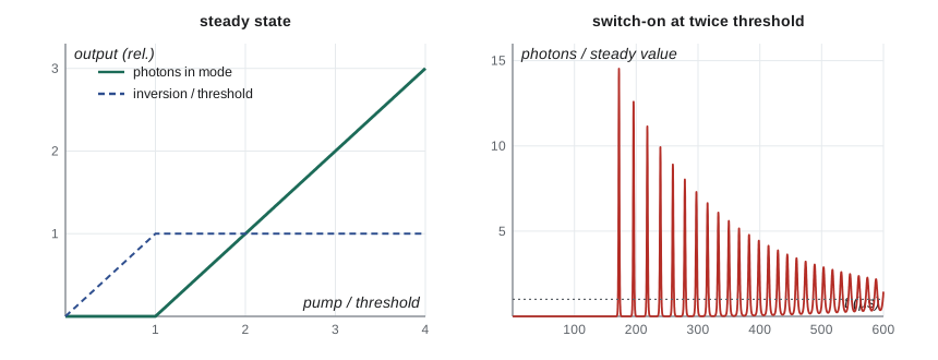
In steady state the time derivatives vanish. Neglecting \(\beta\), the photon equation gives either \(\phi = 0\) or \((c/n)\sigma N = 1/\tau_p\). The first solution is the laser below threshold: no oscillation, and the inversion rises in proportion to the pump, \(N = R_p\tau\). The second solution says that whenever the laser is oscillating, the inversion equals the threshold value, \(N = N_{th} = n/(c\sigma\tau_p)\), regardless of the pump. This is gain clamping. Substituting into the inversion equation gives the photon density,

Above the threshold pump rate \(R_{th}\), every additional inversion created by the pump is immediately converted into a photon by stimulated emission, and the photon number rises linearly with pump rate. This is the characteristic light–current or light–pump curve of a laser, with a sharp kink at threshold. Below threshold the output consists only of weak spontaneous emission; above it, the output rises steeply and becomes directional and narrow-band.

Switching on: spikes and relaxation oscillations

When the pump is switched on suddenly, the photon density is at first almost zero, so stimulated emission is negligible and the inversion rises as \(N(t) = R_p\tau(1 - e^{-t/\tau})\). Nothing much happens until \(N\) passes \(N_{th}\). Then the photon density grows exponentially from the spontaneous seed, but because it starts so small it takes a while to become large, and meanwhile the inversion overshoots well above threshold. When the photons finally become numerous, they consume the excess inversion rapidly, producing an intense spike of light and driving the inversion below threshold. The photons then die away, the inversion recovers, and the cycle repeats with smaller and smaller spikes until the laser settles into its steady state.

Linearizing the rate equations about the steady state shows that small disturbances oscillate at the relaxation frequency

and decay at a rate of about \(r/(2\tau)\). Solid-state lasers, with \(\tau \gg \tau_p\), show pronounced relaxation oscillations at tens to hundreds of kilohertz. Semiconductor lasers, whose carrier lifetime is a few nanoseconds and photon lifetime a few picoseconds, have relaxation frequencies of several gigahertz, which sets the speed at which they can be directly modulated for telecommunications. Gas lasers such as helium–neon have upper-level lifetimes comparable to their photon lifetimes, and their oscillations are strongly damped.

Simulating a laser

The program integrates the rate equations for a Nd:YAG laser with the fourth-order Runge–Kutta method of PHYS-234. It uses \(\tau = 230\) µs, \(\tau_p = 20\) ns and the cross section of lesson 3, switches on the pump at twice threshold, records the time of the first spike and its height, and checks that the photon density settles to the predicted steady value. It then tabulates the steady output against pump rate and computes the threshold gain and slope efficiency of a real rod and cavity.

import math
# Four-level laser rate equations in normalized form
#   dN/dt = P - N/tau - c*sigma*N*Q          (N: inversion density, Q: photon density)
#   dQ/dt = Gamma*c*sigma*N*Q - Q/tau_p + beta*N/tau
tau, tau_p, beta = 230e-6, 20e-9, 1e-8     # upper-level lifetime, photon lifetime, spontaneous fraction into the mode
cs = 3e8 / 1.82 * 2.8e-23                  # (c/n) * sigma for Nd:YAG, m^3/s
Nth = 1 / (cs * tau_p)                     # threshold inversion
Pth = Nth / tau                            # threshold pump rate
print(f"threshold inversion = {Nth:.3e} per m^3, threshold pump rate = {Pth:.3e} per m^3 per s")
def deriv(N, Q, P):
    return P - N / tau - cs * N * Q, cs * N * Q - Q / tau_p + beta * N / tau
def run(P, t_end, dt=4e-9):
    N, Q, t, out = 0.0, 0.0, 0.0, []
    while t < t_end:
        k1 = deriv(N, Q, P); k2 = deriv(N + dt/2*k1[0], Q + dt/2*k1[1], P)
        k3 = deriv(N + dt/2*k2[0], Q + dt/2*k2[1], P); k4 = deriv(N + dt*k3[0], Q + dt*k3[1], P)
        N += dt/6*(k1[0] + 2*k2[0] + 2*k3[0] + k4[0]); Q += dt/6*(k1[1] + 2*k2[1] + 2*k3[1] + k4[1]); t += dt
        out.append((t, N, Q))
    return out
# turn-on at twice threshold: delay, spikes, and settling (relaxation oscillations)
tr = run(2 * Pth, 1.5e-3)
peaks = [tr[i] for i in range(1, len(tr) - 1) if tr[i][2] > tr[i-1][2] and tr[i][2] > tr[i+1][2] and tr[i][2] > 1e15]
Qss = (2 * Pth - Pth) * tau_p           # steady state photon density, Q = (P - Pth) tau_p
print(f"first spike at t = {peaks[0][0]*1e6:.1f} us, height {peaks[0][2]/Qss:.0f} times the steady value")
if len(peaks) > 1:
    T = peaks[1][0] - peaks[0][0]
    print(f"spike spacing at first = {T*1e6:.2f} us")
wR = math.sqrt((2 - 1) / (tau * tau_p))
print(f"small-signal relaxation frequency = {wR/(2*math.pi)/1e3:.1f} kHz, period {2*math.pi/wR*1e6:.2f} us")
late = [x for x in tr if x[0] > 1.4e-3]
print(f"mean photon density, 1.4 to 1.5 ms = {sum(x[2] for x in late)/len(late)/Qss:.3f} of (P - Pth) tau_p")
print(f"inversion at 1.5 ms = {tr[-1][1]/Nth:.4f} of threshold (clamped)")
# output against pump: steady-state Q = (P - Pth) tau_p above threshold
print()
print(f"{'pump / threshold':>17s}{'photons (rel.)':>16s}{'inversion / Nth':>17s}")
for r in (0.5, 0.9, 1.0, 1.5, 2.0, 3.0, 4.0):
    P = r * Pth
    Q = max(0.0, (P - Pth) * tau_p); N = min(P * tau, Nth)
    print(f"{r:17.1f}{Q/(Pth*tau_p):16.2f}{N/Nth:17.2f}")
# threshold gain from mirrors and losses, and slope efficiency
L, R1, R2, alpha = 0.10, 0.999, 0.95, 0.5      # rod length (m), reflectivities, internal loss per m
g_th = alpha + math.log(1 / (R1 * R2)) / (2 * L)
eta_out = math.log(1 / R2) / (math.log(1 / (R1 * R2)) + 2 * alpha * L)
eta_q = 808 / 1064
print()
print(f"threshold gain = {g_th:.3f} per m")
print(f"output-coupling efficiency = {eta_out:.3f}, quantum efficiency 808/1064 = {eta_q:.3f}")
print(f"ideal slope efficiency = {eta_out*eta_q:.3f} (watts out per watt absorbed above threshold)")

threshold inversion = 1.083e+22 per m^3, threshold pump rate = 4.710e+25 per m^3 per s
first spike at t = 172.1 us, height 15 times the steady value
spike spacing at first = 23.58 us
small-signal relaxation frequency = 74.2 kHz, period 13.48 us
mean photon density, 1.4 to 1.5 ms = 1.000 of (P - Pth) tau_p
inversion at 1.5 ms = 0.9999 of threshold (clamped)

 pump / threshold  photons (rel.)  inversion / Nth
              0.5            0.00             0.50
              0.9            0.00             0.90
              1.0            0.00             1.00
              1.5            0.50             1.00
              2.0            1.00             1.00
              3.0            2.00             1.00
              4.0            3.00             1.00

threshold gain = 0.761 per m
output-coupling efficiency = 0.337, quantum efficiency 808/1064 = 0.759
ideal slope efficiency = 0.256 (watts out per watt absorbed above threshold)

The first spike appears 172 µs after the pump is switched on. Most of this delay is the time for the inversion to reach threshold: with the pump at twice threshold, \(N\) reaches \(N_{th} = R_p\tau/2\) at \(t = \tau\ln2 = 159\) µs. The remaining 13 µs is the time for the photon density to grow from the spontaneous seed. The first spike is 15 times higher than the eventual steady output, a reminder that lasers can produce damaging transients when switched on.

The spikes come about 24 µs apart at first, slower than the small-signal relaxation period of 13.5 µs because the early spikes are large and nonlinear; as they shrink, their spacing approaches the linear prediction. By 1.4 ms the laser has settled: the photon density averages exactly \((R_p - R_{th})\tau_p\), and the inversion is clamped at threshold to four decimal places.

Output coupling and slope efficiency

Only the light that passes through the output mirror is useful. Of the photons lost from the cavity, the fraction leaving through mirror 2 is

The output power above threshold is \(P_{out} = \eta_s(P_p - P_{th})\), where the slope efficiency \(\eta_s\) is the product of several factors: the fraction of pump power absorbed, the quantum efficiency \(\nu_{laser}/\nu_{pump}\) (each pump photon can produce at most one laser photon, of lower energy), the fraction of excited ions that contribute to the laser mode rather than to other modes or spontaneous decay, and the output-coupling efficiency \(\eta_{out}\). For the example in the program, a 10 cm rod with internal loss 0.5 per meter and an output mirror of reflectivity 0.95, the threshold gain is 0.76 per meter, about a third of the photons leave through the output mirror, and the ideal slope efficiency is about 0.26. Well-designed diode-pumped lasers reach slope efficiencies of 0.4 to 0.6 by reducing internal loss.

There is an optimum output coupling. If the output mirror is nearly perfect, little light escapes. If it transmits too much, the threshold rises and little pump power is left above threshold. For an output mirror transmission \(T = 1 - R_2\) small compared with one and internal round-trip loss \(L_i\), the maximum output occurs at

where \(g_0\) is the small-signal round-trip gain, \(2\gamma_0\ell\). Typical values for solid-state lasers are a few to ten parts in a hundred; for helium–neon lasers, whose gain is only a few parts in a hundred per pass, output mirrors transmit about one part in a hundred.