Line broadening, gain and population inversion

Lesson 2 treated a transition as if it happened at a single frequency \(\nu_0\). Real transitions absorb and emit over a range of frequencies, the linewidth, and the shape of that range controls almost everything about a laser: how much gain the medium gives at each frequency, how many cavity modes can oscillate, how short a pulse it can produce and how widely it can be tuned. In this lesson we describe line shapes, distinguish homogeneous from inhomogeneous broadening, define the stimulated-emission cross section, and use it to calculate the gain of a population inversion and the inversion a laser needs. We finish with gain saturation, the mechanism that limits how much power any amplifier can deliver.

The line-shape function

The spread of a transition over frequency is described by a normalized line-shape function \(g(\nu)\), with \(\int g(\nu)\,d\nu = 1\). It gives the probability density that a spontaneously emitted photon has frequency \(\nu\), and by Einstein's relations the same function describes absorption and stimulated emission. The rates of lesson 2 become integrals: the stimulated emission rate per atom in a narrow-band field of intensity \(I\) at frequency \(\nu\) is \(B_{21}g(\nu)I/c\) in a medium of unit index. The width of \(g\) is usually quoted as the full width at half maximum (FWHM), \(\Delta\nu\).

Line broadening has two broad classes of cause. In homogeneous broadening, every atom has the same line shape, centered on the same frequency, so the whole collection responds identically. In inhomogeneous broadening, different atoms have their lines centered at different frequencies, and the observed line is the envelope of many narrower lines. The distinction matters greatly in lasers, because a strong field at one frequency affects a homogeneous line everywhere, but an inhomogeneous line only near that frequency.

Homogeneous broadening: the Lorentzian

The most basic broadening is natural, or lifetime, broadening. An excited atom decays with lifetime \(\tau\), so its emitted field decays as \(e^{-t/2\tau}\) and oscillates at \(\nu_0\). The Fourier transform of this damped oscillation is a Lorentzian,

This is the same Lorentzian that described the power absorbed by a damped driven oscillator in PHYS-230, where the full width was the damping rate. Natural widths are small: for a lifetime of 20 ns the width is 8 MHz. Collisions broaden lines further. In a gas, each collision interrupts the phase of the emitted wave, which acts like a shorter effective lifetime and gives a wider Lorentzian; this pressure broadening grows in proportion to the gas pressure. In solids, the dominant homogeneous process at room temperature is the interaction of the ion with lattice vibrations (phonons, PHYS-410), which randomly perturbs the energy levels. For Nd:YAG this gives a homogeneous width of about 120 GHz at room temperature, far larger than its natural width.

Inhomogeneous broadening: the Gaussian

In a gas, atoms move with a Maxwell distribution of velocities. An atom moving with velocity component \(v_z\) toward the observer emits at the Doppler-shifted frequency \(\nu_0(1 + v_z/c)\). Since \(v_z\) has a Gaussian distribution with variance \(k_BT/M\), the line has a Gaussian shape,

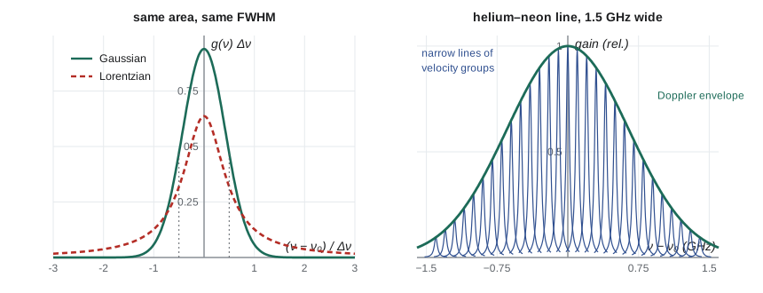
For the neon atoms in a helium–neon laser at about 400 K, the Doppler width is 1.5 GHz, nearly 200 times the natural width. In solids, inhomogeneous broadening arises because ions in different places see slightly different crystal fields. In a crystal such as YAG the sites are nearly identical and this effect is small, but in a glass, where the surroundings vary widely, it dominates. Erbium and ytterbium in silica glass have lines several terahertz wide for this reason, which is what makes them good broadband amplifiers.

When both kinds of broadening are present, the line shape is their convolution, called a Voigt profile. If one width is much larger than the other, the line looks like the wider one near its center, though the Lorentzian always dominates far in the wings because it falls off only as \(1/(\nu - \nu_0)^2\), while the Gaussian falls exponentially.

The stimulated-emission cross section

It is convenient to describe the strength of a transition by an area. The stimulated-emission cross section \(\sigma(\nu)\) is defined so that the stimulated emission rate per atom is \(\sigma(\nu)\,I/(h\nu)\), the cross section times the photon flux. Combining the Einstein relations with the line shape gives

where \(\lambda\) is the vacuum wavelength and \(n\) the refractive index. The peak cross section is largest for strong (large \(A_{21}\)) and narrow (large \(g(\nu_0)\)) transitions. For a line dominated by lifetime broadening, \(g(\nu_0) = 2/(\pi\Delta\nu)\) and \(\Delta\nu = A_{21}/2\pi\), so \(\sigma_{\max} = \lambda^2/(2\pi n^2)\): an isolated atom presents a cross section comparable to the square of the wavelength, enormously larger than its geometric size. Broadening reduces the peak cross section by spreading the same total strength over a wider band.

The gain coefficient of the medium is then

and a weak beam grows as \(I(z) = I(0)e^{\gamma z}\). If \(\Delta N\) is negative, \(\gamma\) is negative and the medium absorbs. The single-pass gain of a medium of length \(\ell\) is \(G = e^{\gamma\ell}\). Gains are often quoted in decibels, \(10\log_{10}G\): a gain coefficient of 2 per meter in a 10 cm rod gives \(G = e^{0.2} = 1.22\).

Computing widths, shapes and gains

The program computes the Doppler width of the helium–neon line, compares Lorentzian and Gaussian shapes of equal width, convolves them numerically to show that the helium–neon line is essentially Gaussian, calculates peak cross sections for helium–neon and Nd:YAG, and finds the inversion needed for a gain of 2 per meter. Finally, it tabulates the gain of ruby, a three-level system, as the excited fraction of chromium ions rises, alongside a hypothetical four-level medium with the same density and cross section.

import math
h, c, kB, amu = 6.62607015e-34, 2.99792458e8, 1.380649e-23, 1.66053906660e-27
# Doppler width of the HeNe line: neon-20 at about 400 K
lam = 632.8e-9; nu0 = c / lam; M = 20 * amu; T = 400
dnu_D = nu0 * math.sqrt(8 * kB * T * math.log(2) / (M * c**2))
print(f"HeNe Doppler FWHM = {dnu_D/1e9:.2f} GHz")
# natural width for a 1 / (2 pi tau) Lorentzian with an effective lifetime of 20 ns
dnu_N = 1 / (2 * math.pi * 20e-9)
print(f"natural FWHM (tau = 20 ns) = {dnu_N/1e6:.1f} MHz")
# line shapes of unit area
def lorentz(x, w): return (w / (2 * math.pi)) / (x * x + (w / 2) ** 2)
def gauss(x, w):
    s = w / (2 * math.sqrt(2 * math.log(2)))
    return math.exp(-x * x / (2 * s * s)) / (s * math.sqrt(2 * math.pi))
def voigt(x, wl, wg, n=4001, span=8):
    # numerical convolution of a Lorentzian and a Gaussian
    s = wg / (2 * math.sqrt(2 * math.log(2))); a = -span * s; dx = 2 * span * s / (n - 1)
    return sum(gauss(a + i * dx, wg) * lorentz(x - a - i * dx, wl) for i in range(n)) * dx
wl, wg = dnu_N, dnu_D
print(f"peak values (1/GHz): Lorentzian {lorentz(0, wg)*1e9:.3f}, Gaussian {gauss(0, wg)*1e9:.3f} (same FWHM)")
print(f"Voigt peak for this line = {voigt(0, wl, wg)*1e9:.4f}, Gaussian alone = {gauss(0, wg)*1e9:.4f}")
for k in (2, 4):
    x = k * wg / 2
    print(f"at {k} half-widths: Lorentzian/Gaussian = {lorentz(x, wg)/gauss(x, wg):.3g}")
# peak stimulated-emission cross section sigma = lam^2 A g(nu0) / (8 pi n^2)
def sigma(lam, A, g0, n=1.0): return lam**2 * A * g0 / (8 * math.pi * n**2)
A21 = 3.4e6
s_he = sigma(lam, A21, gauss(0, dnu_D))
print()
print(f"HeNe cross section = {s_he*1e4:.2e} cm^2")
# Nd:YAG: 1064 nm, tau = 230 us, linewidth about 120 GHz (homogeneous), n = 1.82
s_nd = sigma(1064e-9, 1 / 230e-6, lorentz(0, 120e9), 1.82)
print(f"Nd:YAG cross section = {s_nd*1e4:.2e} cm^2")
print(f"measured Nd:YAG value = 2.8e-19 cm^2, so only {2.8e-19/(s_nd*1e4):.2f} of the decays feed this line")
s_nd = 2.8e-23
# gain coefficient gamma = sigma * dN, and the inversion needed for a gain of 2 per m
for name, s in [('HeNe', s_he), ('Nd:YAG', s_nd)]:
    print(f"{name}: inversion for gain 2 per m = {2/s:.2e} per m^3")
# three-level against four-level: gain as the excited fraction f rises (N atoms per m^3)
N = 1.6e25                       # ruby: Cr ions per m^3
s_ruby = 2.5e-24                 # ruby cross section at 694 nm, m^2
print()
print(f"{'excited fraction':>17s}{'ruby gain (1/m)':>17s}{'four-level gain (1/m)':>23s}")
for f in (0.1, 0.3, 0.5, 0.6, 0.8):
    g3 = s_ruby * N * (2 * f - 1)        # upper minus ground population
    g4 = s_ruby * N * f                   # lower laser level stays empty
    print(f"{f:17.1f}{g3:17.1f}{g4:23.1f}")

HeNe Doppler FWHM = 1.52 GHz
natural FWHM (tau = 20 ns) = 8.0 MHz
peak values (1/GHz): Lorentzian 0.420, Gaussian 0.619 (same FWHM)
Voigt peak for this line = 0.6161, Gaussian alone = 0.6191
at 2 half-widths: Lorentzian/Gaussian = 2.17
at 4 half-widths: Lorentzian/Gaussian = 2.61e+03

HeNe cross section = 3.35e-13 cm^2
Nd:YAG cross section = 3.14e-18 cm^2
measured Nd:YAG value = 2.8e-19 cm^2, so only 0.09 of the decays feed this line
HeNe: inversion for gain 2 per m = 5.96e+16 per m^3
Nd:YAG: inversion for gain 2 per m = 7.14e+22 per m^3

 excited fraction  ruby gain (1/m)  four-level gain (1/m)
              0.1            -32.0                    4.0
              0.3            -16.0                   12.0
              0.5              0.0                   20.0
              0.6              8.0                   24.0
              0.8             24.0                   32.0

The Lorentzian of the same width has a peak only about two-thirds as high as the Gaussian, but at four half-widths from the center it is more than 2,000 times larger. The Voigt peak for the helium–neon line differs from the pure Gaussian by half a part in a hundred, so treating the line as Doppler-broadened is an excellent approximation.

The cross sections differ by more than six orders of magnitude. The neon transition has a cross section of \(3 \times 10^{-13}\ \mathrm{cm^2}\), so an inversion of only \(6 \times 10^{16}\) per cubic meter, a tiny fraction of the gas density, gives a gain of 2 per meter. Nd:YAG has a measured peak cross section of \(2.8 \times 10^{-19}\ \mathrm{cm^2}\). The program's first estimate, using the full upper-level decay rate, comes out about ten times too high, because only about one decay in eleven feeds the particular 1064 nm line: the upper level also decays to other levels and to other crystal-field components. With the measured value, a gain of 2 per meter needs an inversion of \(7 \times 10^{22}\) per cubic meter, about one neodymium ion in 2,000 at the usual doping of one neodymium ion for every hundred yttrium sites, \(1.4 \times 10^{26}\) ions per cubic meter. Solid-state lasers compensate for small cross sections with dense media and long storage times.

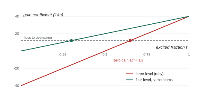
The ruby table shows the three-level penalty directly. With chromium ions at \(1.6 \times 10^{25}\) per cubic meter, the medium absorbs strongly until half the ions are excited, and only then begins to amplify. A four-level medium with the same parameters would already have useful gain at an excited fraction of a tenth.

Gain and threshold

The figure plots the gain coefficient against inversion together with the loss that must be overcome.

A laser oscillates when the round-trip gain balances the round-trip loss. Lesson 5 develops this carefully, but the idea is simple: if light loses a fraction of its power each round trip through mirror transmission, scattering and absorption, the gain must make up exactly that fraction. The inversion at which this happens is the threshold inversion, \(\Delta N_{th}\). Above threshold, the inversion is clamped at \(\Delta N_{th}\): extra pumping goes into more stimulated emission, not into more inversion. This clamping is a consequence of gain saturation.

Gain saturation

As the intensity in the medium grows, stimulated emission depletes the upper level faster than the pump can refill it, and the inversion falls. For a four-level medium with upper-level lifetime \(\tau\), the steady-state inversion in a beam of intensity \(I\) is

where \(\Delta N_0\) is the small-signal inversion produced by the pump alone. The saturation intensity \(I_{sat}\) is the intensity at which stimulated emission removes atoms from the upper level as fast as spontaneous decay does. For Nd:YAG, \(I_{sat} = (1.87 \times 10^{-19})/(2.8 \times 10^{-23} \times 2.3 \times 10^{-4}) = 2.9 \times 10^7\ \mathrm{W/m^2}\), about 2.9 kW per square centimeter. For helium–neon, with its huge cross section, the saturation intensity is only about 10 W per square centimeter.

Saturation behaves differently for the two kinds of broadening. In a homogeneously broadened medium, every atom contributes to gain at every frequency, so a strong field at any frequency reduces the gain across the whole line uniformly. In an inhomogeneously broadened medium, a strong field at frequency \(\nu\) depletes only the atoms resonant near \(\nu\), burning a narrow spectral hole in the gain curve, about one homogeneous width wide, while atoms at other frequencies remain inverted. In a Doppler-broadened gas laser with a standing wave, the field interacts with atoms moving in both directions, burning two holes symmetric about the line center; when the laser is tuned to the center, the two holes merge and the output dips, the Lamb dip, which Willis Lamb predicted in 1964 and which is used to lock lasers to the line center.

These differences explain a basic observation about real lasers. A homogeneously broadened laser tends to oscillate on a single frequency, because the first mode to reach threshold saturates the gain for all the others. An inhomogeneously broadened laser can oscillate on several frequencies at once, each burning its own hole. Lesson 4 counts the cavity modes that fit under a gain curve, and lesson 5 shows how the gain settles at threshold.