Classic experiments I: Millikan oil drop and e/m

The electron was the first elementary particle to be discovered, and two experiments pinned down its properties: J. J. Thomson's measurement of its charge-to-mass ratio in 1897, and Robert Millikan's measurement of its charge between 1909 and 1913. Both are still performed in teaching laboratories, and both repay study not only for their physics but for what they show about experimental method, including, in Millikan's case, an instructive controversy about how data are selected. This lesson works through the physics of each experiment, simulates them, and extracts the elementary charge and the charge-to-mass ratio from the simulated data.

Thomson and the charge-to-mass ratio

By the 1890s physicists knew that an electric discharge in a partly evacuated tube produced cathode rays, but not whether these were waves in the ether or streams of particles. In 1897 J. J. Thomson at the Cavendish Laboratory in Cambridge showed that the rays were deflected by both electric and magnetic fields, and that the ratio of the deflections gave the ratio of charge to mass of the carriers. He found the same value whatever gas filled the tube and whatever metal formed the cathode, and the value was about a thousand times larger than the charge-to-mass ratio of the hydrogen ion known from electrolysis. Thomson concluded that cathode rays were made of particles, which he called corpuscles, far lighter than atoms and common to all matter. He received the Nobel Prize in 1906.

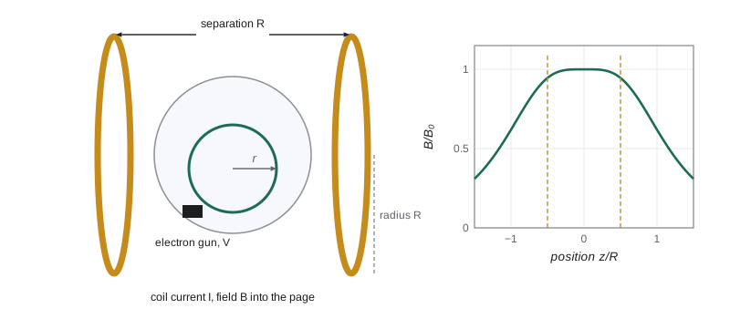
The teaching version of the experiment uses a glass bulb filled with low-pressure gas, an electron gun that accelerates electrons through a potential difference \(V\), and a pair of Helmholtz coils that produce a uniform magnetic field \(B\) perpendicular to the beam. The electrons gain kinetic energy \(\tfrac12mv^2 = eV\). In the magnetic field the Lorentz force \(evB\) acts at right angles to the velocity, so the electrons move in a circle of radius \(r\) given by \(evB = mv^2/r\). The beam excites the gas, which glows faintly along its path, so the circle is visible and its diameter can be measured. Eliminating \(v\) between the two equations gives

The field at the center of a pair of Helmholtz coils, each of \(N\) turns and radius \(R\), separated by \(R\) and carrying current \(I\) in the same sense, is

found by adding the on-axis fields of two loops at distance \(R/2\) from the midpoint, \(\mu_0NIR^2/[2(R^2 + R^2/4)^{3/2}]\) each. The spacing \(R\) is chosen because it makes the second derivative of the field vanish at the center, so the field is uniform to within about 1 part in 100 over a region a third of the coil radius across. PHYS-381 derives the loop field; here we use the result.

The uncertainty budget is instructive. The fractional uncertainty in \(e/m\) is the quadrature sum of the uncertainty in \(V\), twice that in \(B\) and twice that in \(r\). Measuring the beam diameter by eye against a scale behind the bulb is the weak point: parallax, the width of the glowing beam and the difficulty of finding the center of the circle give uncertainties of a few parts in 100. Two systematic effects also enter. The Earth's magnetic field, about 50 μT, is a few parts in 100 of the coil field and must be canceled by orienting the apparatus or measured and subtracted. And electrons do not all leave the gun with exactly \(eV\): contact potentials and the gun geometry shift their energy. Taking several combinations of \(V\) and \(I\) and fitting \(r^2\) against \(2V/B^2\) separates such offsets from the slope.

Millikan and the elementary charge

The charge-to-mass ratio did not determine the charge itself. Several groups had tried to measure it by watching clouds of charged water droplets fall, but evaporation made the results unreliable. In 1909 Robert Millikan, with his graduate student Harvey Fletcher, who suggested using oil instead of water, began observing single tiny oil drops between two horizontal metal plates. A drop is charged by friction when sprayed, or by ionizing the air with X-rays or a radioactive source. With no voltage on the plates, the drop falls under gravity; drag from the air quickly brings it to a steady terminal speed. With a voltage on the plates, the electric force can make it rise. Timing the drop over a fixed distance, with and without the field, gives its charge.

For a sphere of radius \(a\) moving slowly through air of viscosity \(\eta\), George Gabriel Stokes showed in 1851 that the drag force is \(6\pi\eta av\). With the field off, gravity minus buoyancy balances drag at the fall speed \(v_f\); neglecting the small buoyancy of air,

So the fall speed gives the radius of the drop, which is far too small to measure directly, about a micrometer. With the field \(E = V/d\) on and the drop rising at speed \(v_r\), the electric force \(qE\) balances gravity plus drag: \(qE = mg + 6\pi\eta av_r = 6\pi\eta a(v_f + v_r)\). Therefore

Millikan found that every charge he measured, on drops of different sizes and even on the same drop as it picked up or lost charge, was an integer multiple of a single value. His 1913 result was \(e = 1.592 \times 10^{-19}\) C. The modern value, fixed exactly since 2019 as part of the definition of the ampere, is \(1.602176634 \times 10^{-19}\) C. Millikan's value was low by about 0.6 parts in 100 because he used a value of the viscosity of air that was itself slightly wrong, a systematic error unrelated to his technique. It was corrected in the 1930s when X-ray crystal measurements of Avogadro's number gave an independent value.

Stokes's law needs one correction for drops this small. Their radius approaches the mean free path of air molecules, about 70 nm, and the air no longer behaves as a continuous fluid, so the drag is somewhat less than \(6\pi\eta av\). Millikan applied the Cunningham correction, multiplying the viscosity by \(1/(1 + b/(pa))\) with an empirical constant \(b\) and the pressure \(p\). For micrometer drops at atmospheric pressure the correction is several parts in 100, larger than the statistical errors, so a precise result must include it. Our simulation leaves it out, which is why it uses plain Stokes drag both to generate and to analyze the data.

The Millikan controversy

Millikan's notebooks, studied by the historian Gerald Holton in 1978, show that he recorded measurements on roughly 140 drops in the relevant period but published results from 58, while stating in his 1913 paper that the published drops were not a selected group. Some readers concluded that he had discarded drops whose charges did not fit his hypothesis of a single unit charge. Later analyses, notably by the philosopher Allan Franklin, found that most excluded drops were rejected for reasons Millikan noted at the time, such as drops that were too large or too small for Stokes's law to apply, apparatus problems or runs before the apparatus was working well; and that including them would not have changed his value of \(e\) significantly, though it would have increased the stated uncertainty. The episode is now taught as a lesson in two directions. Experimenters must be free to reject data for good reasons, documented at the time and decided by criteria that do not depend on the result. And a paper must say honestly what was done. We return to this in lesson 11.

Extracting e from the data

Given a list of charges, how do we find the unit? Millikan computed differences between successive charges on the same drop and looked for their greatest common divisor. With many drops of different charges, a cleaner method is to scan candidate unit charges \(u\) and, for each, measure how far every charge lies from the nearest integer multiple, \(\sum(q_i/u - \text{round}(q_i/u))^2\). The true unit makes every term small. One subtlety: \(u/2\), \(u/3\) and so on also make the terms small, since every multiple of \(e\) is also a multiple of \(e/2\). The scan must therefore start above half the expected value, or the search must prefer the largest unit that fits. Once each drop's integer \(n_i\) is assigned, the best estimate is \(e = \sum q_i/\sum n_i\).

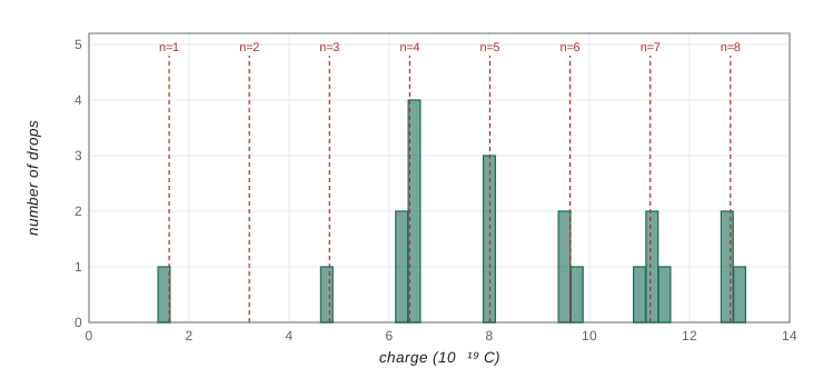
The program simulates the experiment with plates 6 mm apart at 500 V, oil of density 886 kg/m\(^3\), drops of radius between 0.6 and 1.4 μm carrying between one and eight elementary charges, and a 1.5 parts in 100 timing scatter in each speed. It discards drops that the field cannot lift, as the experimenter would, then scans for the unit charge. It finishes with three settings of the Thomson apparatus, using coils of 130 turns and 15 cm radius.

import math, random
random.seed(397)
e_true = 1.602176634e-19
eta, rho, g = 1.83e-5, 886.0, 9.81          # air viscosity (Pa s), oil density (kg/m^3)
d, V = 6.0e-3, 500.0; E = V/d               # plate gap 6 mm, 500 V
# 1. Simulate 25 drops: random radius near 1 micron, random small charge, 1.5 % timing scatter in each speed.
drops = []
for _ in range(25):
    a = random.uniform(0.6e-6, 1.4e-6); n = random.randint(1, 8)
    vf = 2*rho*g*a*a/(9*eta)                         # terminal fall speed, field off (Stokes drag)
    vr = n*e_true*E/(6*math.pi*eta*a) - vf           # rise speed, field on
    if vr <= 0: continue
    drops.append((vf*random.gauss(1, 0.015), vr*random.gauss(1, 0.015)))
qs = []
for vf, vr in drops:
    a = math.sqrt(9*eta*vf/(2*rho*g))
    qs.append(6*math.pi*eta*a*(vf + vr)/E)
print(f"{len(qs)} drops; measured charges (units of 1e-19 C):", " ".join(f"{q*1e19:.2f}" for q in sorted(qs)))
# 2. Find the elementary charge: the unit that makes every charge closest to an integer multiple.
def badness(u): return sum((q/u - round(q/u))**2 for q in qs)
best = min((badness(u*1e-21), u*1e-21) for u in range(120, 200))   # scan 1.20e-19 .. 1.99e-19 C
u = best[1]
ns = [round(q/u) for q in qs]
e_fit = sum(q for q in qs)/sum(ns)
spread = math.sqrt(sum((q/n - e_fit)**2 for q, n in zip(qs, ns))/(len(qs) - 1))
print(f"best unit from the scan {u:.3e} C; refined e = {e_fit:.4e} C, scatter per drop {spread:.1e} C, standard error {spread/math.sqrt(len(qs)):.1e} C")
print(f"accepted value 1.602177e-19 C; difference {(e_fit/e_true - 1)*100:+.2f} parts per hundred")
# 3. e/m from an electron beam bent into a circle in a Helmholtz pair (N = 130 turns, R = 0.150 m).
mu0 = 4e-7*math.pi; N, Rc = 130, 0.150
for Vacc, I, r in ((250.0, 1.50, 0.0458), (300.0, 1.80, 0.0414), (350.0, 2.10, 0.0386)):
    B = (4/5)**1.5*mu0*N*I/Rc
    print(f"V = {Vacc:.0f} V, I = {I:.2f} A: B = {B*1e3:.3f} mT, r = {r*100:.2f} cm, e/m = {2*Vacc/(B*B*r*r):.3e} C/kg")
print(f"accepted e/m = {e_true/9.1093837e-31:.3e} C/kg")

21 drops; measured charges (units of 1e-19 C): 1.62 4.79 6.25 6.33 6.40 6.41 6.48 6.49 7.98 8.02 8.09 9.40 9.62 9.76 11.10 11.16 11.20 11.55 12.67 12.86 12.91
best unit from the scan 1.600e-19 C; refined e = 1.6025e-19 C, scatter per drop 2.0e-21 C, standard error 4.4e-22 C
accepted value 1.602177e-19 C; difference +0.02 parts per hundred
V = 250 V, I = 1.50 A: B = 1.169 mT, r = 4.58 cm, e/m = 1.744e+11 C/kg
V = 300 V, I = 1.80 A: B = 1.403 mT, r = 4.14 cm, e/m = 1.779e+11 C/kg
V = 350 V, I = 2.10 A: B = 1.637 mT, r = 3.86 cm, e/m = 1.754e+11 C/kg
accepted e/m = 1.759e+11 C/kg

Twenty-one drops survive. Their charges cluster clearly near integer multiples of \(1.6 \times 10^{-19}\) C, with no drop anywhere in between. The scan picks the unit \(1.600 \times 10^{-19}\) C, and the refined value is \(e = 1.6025 \times 10^{-19}\) C, within 0.02 parts in 100 of the true value. The scatter of single drops, \(2.0 \times 10^{-21}\) C or about 1.2 parts in 100, comes from the timing noise; the standard error of the mean is a quarter of that. The \(e/m\) values from three settings are 1.744, 1.779 and \(1.754 \times 10^{11}\) C/kg, with a mean of \(1.759 \times 10^{11}\) C/kg, matching the accepted value. Their spread of about 1 part in 100 reflects a radius read to half a millimeter on circles of about 4 cm.