Data acquisition, sampling and lock-in detection

Today almost every experiment records its data with a computer. An analog-to-digital converter turns a voltage into numbers, many thousands or millions of times a second, and software does the rest. This brings enormous power, and new ways to go wrong. This lesson covers the essentials of digitizing signals: resolution and quantization, the sampling theorem and aliasing, and the anti-aliasing filter. It then describes one of the most powerful techniques in experimental physics, phase-sensitive or lock-in detection, which can recover a signal thousands of times smaller than the noise accompanying it, and ends with practical advice on recording and keeping data.

Analog-to-digital conversion

An analog-to-digital converter, or ADC, compares its input with a reference voltage and outputs an integer. An \(n\)-bit converter divides its range into \(2^n\) steps: a 12-bit converter on a 10 V range has steps of 2.4 mV; a 16-bit one, 0.15 mV; a 24-bit converter, as used in precision voltmeters and audio, about 0.6 μV. Rounding to the nearest step adds quantization error, which behaves like noise uniformly distributed over one step \(q\), with rms value \(q/\sqrt{12}\). A converter's useful resolution is usually less than its nominal number of bits, because its own noise and nonlinearity exceed one step; the specification called effective number of bits measures what you actually get. To use the resolution well, amplify the signal so that it nearly fills the converter's range without exceeding it. A signal that overloads the converter is clipped, and the clipping produces spurious frequencies that no later processing can remove.

The sampling theorem

A converter samples the signal at discrete times, every \(1/f_s\). What can such samples tell us? The sampling theorem, stated by Harry Nyquist in 1928 and proved by Claude Shannon in 1949, says that a signal containing no frequencies above \(f_{\max}\) is completely determined by samples taken at a rate \(f_s > 2f_{\max}\). Half the sampling rate, \(f_s/2\), is the Nyquist frequency. Sampling faster than twice the highest frequency loses nothing; sampling slower loses information in a particularly treacherous way.

The reason is that sinusoids at frequencies \(f\) and \(f_s - f\), or more generally \(|f - kf_s|\) for any integer \(k\), produce exactly the same samples. Write a sample of \(\sin(2\pi ft)\) at \(t = n/f_s\): replacing \(f\) by \(f_s - f\) gives \(\sin(2\pi n - 2\pi fn/f_s) = -\sin(2\pi fn/f_s)\), the same samples with opposite sign. A 900 Hz tone sampled 1000 times per second is indistinguishable from a 100 Hz tone. This is aliasing. Once the samples are taken, no analysis can tell the two apart, so aliased noise or interference appears at a false frequency inside the band of interest, where it may be mistaken for a real effect. The same thing makes wagon wheels in films appear to turn slowly backwards: the film camera samples their motion at 24 frames per second.

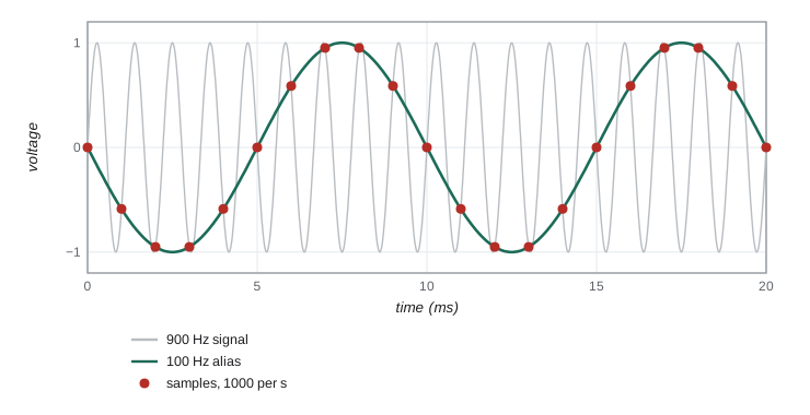
The cure is to remove the high frequencies before sampling with an analog low-pass filter, the anti-aliasing filter, whose corner lies below the Nyquist frequency and which attenuates strongly above it. Practical systems sample comfortably faster than twice the highest frequency of interest, often five to ten times, so that the filter's roll-off has room to work. Digital filtering after sampling cannot replace the analog filter, because by then the alias has already landed inside the band.

Spectra from data

The discrete Fourier transform turns \(N\) samples into the amplitudes of \(N/2\) frequency components spaced by \(f_s/N\), from zero up to the Nyquist frequency. Computed by the fast Fourier transform algorithm of James Cooley and John Tukey, published in 1965, it is the basic tool for finding periodicities, measuring noise spectra and diagnosing interference: mains pickup appears as a sharp line at 60 Hz and its harmonics. Two practical points matter. The frequency resolution is the inverse of the record length, so resolving two lines 0.1 Hz apart needs at least 10 s of data. And unless the record contains a whole number of cycles, energy leaks into neighboring frequency bins; multiplying the data by a smooth window function, such as the Hann window, reduces this leakage at the cost of a slightly broader peak. PHYS-234 implemented the fast Fourier transform; here we use a plain discrete transform to show aliasing.

Lock-in detection

Suppose the signal you want is tiny and steady, far smaller than the noise. Lesson 6 showed that narrowing the bandwidth helps, but at DC you meet flicker noise and drifts. The lock-in idea, developed in the 1940s and associated especially with Robert Dicke at the MIT Radiation Laboratory and later Princeton, is to move the signal to a frequency of your choosing, away from the \(1/f\) noise and from interference, and then to detect it with an extremely narrow filter centered exactly on that frequency. You modulate the signal at a reference frequency \(f_r\), by chopping a light beam with a rotating slotted wheel, by switching a voltage, by oscillating a magnetic field. The detector output then contains a component \(A\sin(2\pi f_rt + \phi)\) plus noise.

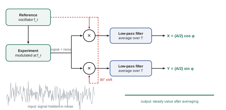
The lock-in amplifier multiplies this input by a reference sine wave at exactly \(f_r\), supplied by the same oscillator that drives the modulation, and averages the product. Using \(\sin a\sin b = \tfrac12[\cos(a - b) - \cos(a + b)]\),

The product has a steady part proportional to \(A\cos\phi\) and a part at twice the frequency, which averaging removes. Noise at any frequency \(f\) far from \(f_r\) is shifted to \(|f - f_r|\) and \(f + f_r\), which also average away. Only noise within roughly \(1/T\) of the reference frequency survives an average over a time \(T\). Multiplying by the cosine as well gives \((A/2)\sin\phi\); combining the two outputs, called X and Y, gives the amplitude \(A\) and the phase \(\phi\) separately. The effective bandwidth of the measurement is set by the averaging time, not by the electronics, and can be a fraction of a hertz centered on a reference of several kilohertz. A lock-in is equivalent to a band-pass filter with a quality factor of a million that automatically tracks the reference.

The program simulates a 2.0 μV signal at 1 kHz, with a phase of 30 degrees, buried in 100 μV rms of white noise, an input signal-to-noise ratio of about 0.014. It records 20 s of data at 50,000 samples per second and applies the lock-in algorithm. Before that, it shows aliasing: tones at 900 Hz and 1100 Hz sampled at 1000 per second both appear at 100 Hz, while sampling at 4000 per second shows the 900 Hz tone correctly.

import math, cmath, random
random.seed(397)
# 1. Aliasing: a 900 Hz tone sampled at 1000 samples per second appears at 100 Hz.
def dft_peak(x, fs):
    N = len(x); best = (0, 0)
    for k in range(1, N//2):
        X = sum(x[n]*cmath.exp(-2j*math.pi*k*n/N) for n in range(N))
        if abs(X) > best[0]: best = (abs(X), k*fs/N)
    return best[1]
for f, fs in ((100, 1000), (400, 1000), (900, 1000), (1100, 1000), (900, 4000)):
    x = [math.sin(2*math.pi*f*n/fs) for n in range(200)]
    print(f"tone {f:5d} Hz sampled at {fs:5d} per s (Nyquist {fs//2} Hz): spectrum peak at {dft_peak(x, fs):6.1f} Hz")
# 2. Lock-in detection: a 2.0 microvolt signal at 1 kHz buried in 100 microvolts rms of white noise.
fs, fref, A = 50000, 1000.0, 2.0e-6
phase = math.radians(30)
noise = 100e-6
N = 1000000                      # 20 s of data
X = Y = 0.0
for n in range(N):
    t = n/fs
    v = A*math.sin(2*math.pi*fref*t + phase) + random.gauss(0, noise)
    X += v*math.sin(2*math.pi*fref*t); Y += v*math.cos(2*math.pi*fref*t)
X *= 2/N; Y *= 2/N               # mixing and averaging (an ideal low-pass filter over 20 s)
print(f"lock-in output: amplitude {math.hypot(X, Y)*1e6:.2f} microvolts, phase {math.degrees(math.atan2(Y, X)):.1f} degrees (true 2.00, 30.0)")
print(f"expected noise in each output: {noise*math.sqrt(2/N)*1e6:.2f} microvolts; input SNR {A/math.sqrt(2)/noise:.4f}")

tone   100 Hz sampled at  1000 per s (Nyquist 500 Hz): spectrum peak at  100.0 Hz
tone   400 Hz sampled at  1000 per s (Nyquist 500 Hz): spectrum peak at  400.0 Hz
tone   900 Hz sampled at  1000 per s (Nyquist 500 Hz): spectrum peak at  100.0 Hz
tone  1100 Hz sampled at  1000 per s (Nyquist 500 Hz): spectrum peak at  100.0 Hz
tone   900 Hz sampled at  4000 per s (Nyquist 2000 Hz): spectrum peak at  900.0 Hz
lock-in output: amplitude 1.98 microvolts, phase 34.8 degrees (true 2.00, 30.0)
expected noise in each output: 0.14 microvolts; input SNR 0.0141

The lock-in recovers an amplitude of \(1.98\) μV and a phase of 35 degrees. The expected noise in each output after 20 s is about 0.14 μV, so the amplitude agrees with the true 2.00 μV within its uncertainty; the phase error of 5 degrees corresponds to the same small noise acting on the Y channel, about 0.14/2 radians. The signal was 70 times smaller than the noise in the raw data and is now measured to about 7 parts in 100. Longer averaging would improve it further as \(1/\sqrt{T}\). Real lock-in amplifiers do exactly this, digitally, and are standard in optics, condensed matter physics and any experiment where a small modulated signal must be pulled out of noise.

Timing and synchronization

Many measurements depend on knowing exactly when each sample was taken. A converter's sampling clock is a crystal oscillator, accurate to perhaps 20 parts per million, which is fine for audio but not for comparing data from two instruments over hours: two clocks that differ by 20 parts per million drift apart by 72 ms per hour. Experiments that combine data from several digitizers therefore share a common clock or a common trigger, or timestamp their data against a reference such as a rubidium oscillator or the time signals broadcast by the Global Positioning System, which carry the accuracy of atomic clocks to any receiver. Jitter, the random variation in the moment a sample is taken, adds noise in proportion to how fast the signal is changing: sampling a 1 MHz sine wave of 1 V amplitude with 1 ns of jitter adds about 6 mV of error at its steepest point. For fast signals, the quality of the clock can matter as much as the number of bits.

Recording and keeping data

The data from an experiment are its most valuable product, and they deserve care. Record raw data, not only processed values; you cannot later undo a smoothing or a subtraction that turns out to be wrong. Keep a laboratory notebook, on paper or electronic, written as you go, dated, with every setting, every change to the apparatus and every surprise, including the runs that failed. Record the units and the instrument used for each quantity. Store the analysis code with the data, under version control, so that every figure in a report can be regenerated from the raw files. Back up. Many research funders and journals now require data to be preserved and, where possible, shared, following principles often summarized as findable, accessible, interoperable and reusable. Lesson 11 returns to why this matters for reproducibility.