Uncertainty II: fitting, chi-squared and model comparison

Most experiments produce not one number but a set of points: period against length, resistance against temperature, stopping voltage against frequency. The physics lies in a model that should describe them, a line, a power law, an exponential decay, with parameters to be determined. This lesson develops weighted least squares fitting from the principle of maximum likelihood, shows how to get the uncertainties of the fitted parameters, introduces the chi-squared statistic and its probability as a test of whether the model fits, and compares competing models with the Akaike information criterion. PHYS-234 implemented least squares and the fast Fourier transform as numerical methods; here the focus is on the statistical meaning of a fit and on the judgment needed to use it well.

From likelihood to least squares

Suppose we measure \(y_i\) at known \(x_i\), each with a normally distributed uncertainty \(\sigma_i\), and a model predicts \(y = f(x; \mathbf{a})\) with parameters \(\mathbf{a}\). If the model and parameters are right, the probability of obtaining the observed data is the product of normal distributions,

where

The principle of maximum likelihood says that the best parameters are those that make the observed data most probable. Because the probability is \(e^{-\chi^2/2}\), maximizing it means minimizing \(\chi^2\): this is weighted least squares. Each residual is measured in units of its own uncertainty, so precise points pull harder on the fit. When all uncertainties are equal, the weights drop out and we recover ordinary least squares. Adrien-Marie Legendre published the method in 1805 and Carl Friedrich Gauss, who claimed to have used it since 1795, justified it with the normal distribution in 1809.

The straight line

For \(f = a + bx\), set \(\partial\chi^2/\partial a = \partial\chi^2/\partial b = 0\). With weights \(w_i = 1/\sigma_i^2\), define \(S = \sum w_i\), \(S_x = \sum w_ix_i\), \(S_y = \sum w_iy_i\), \(S_{xx} = \sum w_ix_i^2\), \(S_{xy} = \sum w_ix_iy_i\) and \(\Delta = SS_{xx} - S_x^2\). The two conditions are linear equations whose solution is

The parameter uncertainties follow by propagating the \(\sigma_i\) through these formulas, since \(a\) and \(b\) are linear combinations of the \(y_i\). The intercept and slope are generally correlated, with covariance \(-S_x/\Delta\); if you later compute something from both, such as the value of the line at some \(x\), you need the covariance. Centering the \(x\) values at their weighted mean removes the correlation. The same approach works for any model that is linear in its parameters, such as a polynomial: the normal equations become a small matrix equation \(\mathbf{A}\mathbf{a} = \mathbf{b}\), where \(\mathbf{A}\) is called the curvature matrix, and the inverse \(\mathbf{A}^{-1}\) is the covariance matrix of the fitted parameters. Its diagonal elements are the parameter variances. For models that are nonlinear in their parameters, such as \(y = A e^{-x/\tau}\), the minimum must be found iteratively, but near the minimum the same curvature matrix gives the uncertainties.

Does the model fit? Chi-squared

A fit always produces parameters, even when the model is wrong. The value of \(\chi^2\) at the minimum tells us whether the model is plausible. If the model is right and the uncertainties are correct, each term \((y_i - f_i)/\sigma_i\) behaves like a standard normal variable, so each contributes about 1 on average. Fitting \(m\) parameters to \(N\) points uses up \(m\) degrees of freedom, leaving \(\nu = N - m\). The expected value of \(\chi^2\) is \(\nu\), with standard deviation \(\sqrt{2\nu}\). The reduced chi-squared \(\chi^2/\nu\) should therefore be close to 1:

much larger than 1 means the model does not fit, or the uncertainties are underestimated; much smaller than 1 means the uncertainties are overestimated, or, more worrying, that the data have been smoothed, selected or copied. The precise statement uses the chi-squared distribution: the probability of getting a value at least as large as the one observed, if the model is right, is

where \(Q\) is the regularized upper incomplete gamma function. A p-value of 0.3 is unremarkable; 0.01 is suspicious; \(10^{-6}\) means the model is wrong. A p-value near 1 means the fit is too good to be true. Remember that chi-squared tests the model and the uncertainties together: a perfectly good model will fail if the error bars are too small.

Residuals

Always plot the residuals, \(y_i - f(x_i)\), or better the normalized residuals \((y_i - f_i)/\sigma_i\), against \(x\). If the model is right, they scatter randomly about zero, about two thirds within \(\pm 1\). A systematic pattern, an arch, a slope, a trend at one end, reveals a missing term in the model even when chi-squared alone is ambiguous, and suggests what the missing term is. Residual plots are one of the cheapest and most powerful diagnostics in data analysis.

An example: a platinum resistance thermometer

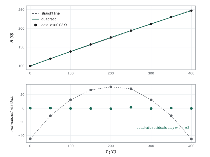
Platinum resistance thermometers are the standard for precise temperature measurement between about \(-200\) and \(+660\) °C. Their resistance follows the Callendar–Van Dusen equation, which above 0 °C is \(R = R_0(1 + AT + BT^2)\), with a small negative \(B\). The program simulates nine readings of a 100 Ω sensor from 0 to 400 °C, each with an uncertainty of 0.03 Ω, and fits both a straight line and a quadratic. It solves the normal equations by Gauss–Jordan elimination, which also gives the covariance matrix, and computes the p-value with a stdlib implementation of the incomplete gamma function.

import math, random
random.seed(397)
def gammq(a, x):
    """Upper regularized incomplete gamma Q(a, x): series for x < a + 1, continued fraction otherwise."""
    gl = math.lgamma(a)
    if x < a + 1:
        ap, s, d = a, 1/a, 1/a
        for _ in range(500):
            ap += 1; d *= x/ap; s += d
            if abs(d) < abs(s)*1e-15: break
        return 1 - s*math.exp(-x + a*math.log(x) - gl)
    b = x + 1 - a; c = 1e300; d = 1/b; h = d
    for i in range(1, 500):
        an = -i*(i - a); b += 2
        d = an*d + b; d = 1e-300 if abs(d) < 1e-300 else d
        c = b + an/c; c = 1e-300 if abs(c) < 1e-300 else c
        d = 1/d; dl = d*c; h *= dl
        if abs(dl - 1) < 1e-15: break
    return math.exp(-x + a*math.log(x) - gl)*h
def wfit(xs, ys, ss, deg):
    """Weighted least squares polynomial fit via normal equations; returns parameters, errors, chi-squared."""
    k = deg + 1
    A = [[sum(x**(i + j)/s**2 for x, s in zip(xs, ss)) for j in range(k)] for i in range(k)]
    b = [sum(y*x**i/s**2 for x, y, s in zip(xs, ys, ss)) for i in range(k)]
    n = k; M = [row[:] + [1.0 if r == c else 0.0 for c in range(n)] for r, row in enumerate(A)]
    for c in range(n):                                   # Gauss-Jordan inverse of the curvature matrix
        p = max(range(c, n), key=lambda r: abs(M[r][c])); M[c], M[p] = M[p], M[c]
        piv = M[c][c]; M[c] = [v/piv for v in M[c]]
        for r in range(n):
            if r != c:
                f = M[r][c]; M[r] = [a - f*bb for a, bb in zip(M[r], M[c])]
    cov = [row[n:] for row in M]
    par = [sum(cov[i][j]*b[j] for j in range(n)) for i in range(n)]
    chi2 = sum(((y - sum(par[i]*x**i for i in range(k)))/s)**2 for x, y, s in zip(xs, ys, ss))
    return par, [math.sqrt(cov[i][i]) for i in range(n)], chi2
# Platinum resistance thermometer: R(T) = R0 (1 + A T + B T^2), R0 = 100 ohm, A = 3.9083e-3, B = -5.775e-7.
Ts = [0, 50, 100, 150, 200, 250, 300, 350, 400]
sig = [0.03]*len(Ts)
Rs = [100*(1 + 3.9083e-3*T - 5.775e-7*T*T) + random.gauss(0, 0.03) for T in Ts]
for deg in (1, 2):
    par, err, chi2 = wfit(Ts, Rs, sig, deg)
    dof = len(Ts) - (deg + 1)
    aic = chi2 + 2*(deg + 1)
    print(f"degree {deg}: chi2 = {chi2:9.2f} for {dof} dof, reduced {chi2/dof:8.2f}, p = {gammq(dof/2, chi2/2):.3g}, AIC = {aic:.1f}")
    print("   parameters:", ", ".join(f"{p:.6g} +/- {e:.2g}" for p, e in zip(par, err)))
par, err, chi2 = wfit(Ts, Rs, sig, 2)
print(f"fitted A = {par[1]/par[0]:.5e} per degree, B = {par[2]/par[0]:.3e} per degree squared")

degree 1: chi2 =   7051.25 for 7 dof, reduced  1007.32, p = 0, AIC = 7055.3
   parameters: 101.357 +/- 0.018, 0.367758 +/- 7.7e-05
degree 2: chi2 =      3.06 for 6 dof, reduced     0.51, p = 0.801, AIC = 9.1
   parameters: 100.018 +/- 0.024, 0.390719 +/- 0.00028, -5.74043e-05 +/- 6.8e-07
fitted A = 3.90649e-03 per degree, B = -5.739e-07 per degree squared

Plotted, the straight line looks like a reasonable fit: the curvature amounts to only about 1 Ω out of 160. But chi-squared exposes it immediately: 7051 for 7 degrees of freedom, a reduced chi-squared above 1000 and a p-value that underflows to zero. The residual plot shows why, a clear arch. The quadratic gives \(\chi^2 = 3.06\) for 6 degrees of freedom, a p-value of 0.80, and recovers the coefficients \(A = 3.906 \times 10^{-3}\) per degree and \(B = -5.74 \times 10^{-7}\) per degree squared, close to the standard values for industrial platinum sensors, \(3.9083 \times 10^{-3}\) and \(-5.775 \times 10^{-7}\).

Comparing models

Adding parameters always lowers chi-squared, so a lower \(\chi^2\) alone does not prove a more complicated model is better. A ninth-degree polynomial passes exactly through nine points and has \(\chi^2 = 0\), but it is useless for interpolation and tells us nothing about physics. Several tools balance goodness of fit against complexity. The simplest is to look at the change in \(\chi^2\) when one parameter is added: if the simpler model is correct, the drop behaves like a chi-squared variable with one degree of freedom, so a drop much larger than about 4 is significant. The Akaike information criterion, introduced by Hirotugu Akaike in 1974, is \(\text{AIC} = \chi^2 + 2m\) for a model with \(m\) parameters; the model with the lowest AIC is preferred, and a difference of more than about 10 is decisive. Here the AIC falls from 7055 to 9.1, overwhelmingly favoring the quadratic. A cubic term would lower chi-squared slightly but raise the AIC, because it fits noise rather than signal.

Physics should guide the choice as much as statistics. The quadratic is not merely a better curve: it is the form predicted for platinum by the physics of electron scattering and adopted in the international standard. Choosing a model because it has theoretical grounds, and then testing it, is far stronger than searching through many functions for the one that fits best. That search inflates the apparent significance, a theme we return to in lesson 11.

Fitting when x also has errors

The derivation above assumed the \(x_i\) are known exactly. When they have uncertainties \(\sigma_{x,i}\) too, a common fix is the effective variance method: replace \(\sigma_i^2\) by \(\sigma_{y,i}^2 + (f'(x_i)\,\sigma_{x,i})^2\), which projects the \(x\) error onto the \(y\) direction through the slope of the model. Iterate, since the slope depends on the fit. If the \(x\) errors dominate, swap the roles of the variables. More rigorous methods, such as orthogonal distance regression, minimize the distance perpendicular to the curve, scaled by both uncertainties.