Designing an experiment: variables, controls and scaling

An experiment is designed before it is built. The hours spent thinking about what to vary, what to hold fixed, what precision is needed and what could go wrong are the cheapest hours in the whole project, and they decide whether the expensive hours at the bench produce an answer. This lesson sets out the main ideas of experimental design for physics: identifying variables and controlling the rest, using dimensional analysis and scaling to decide what to measure, choosing the range and spacing of data, estimating in advance the number of repeats you will need, and running a pilot experiment before committing to the real one.

Variables and controls

Most experiments ask how one quantity depends on another. The quantity you set is the independent variable: the length of a pendulum, the voltage on a capacitor, the wavelength of light falling on a photocathode. The quantity you measure in response is the dependent variable: the period, the charge, the stopping voltage. Everything else that could affect the result is a potential confounding variable, and the design must either hold it fixed, measure it so that it can be corrected for, or randomize it so that its effects average out rather than masquerade as a trend.

In a pendulum experiment, the confounding variables include the amplitude, the temperature (which changes the string length slightly), air currents, the flexibility of the support and the size of the bob. You can hold amplitude fixed by always releasing from the same angle, measure temperature, shield the pendulum from moving air and choose a rigid clamp. Randomization matters when a variable drifts with time: if the room warms up through the afternoon and you measure the long pendulums last, a temperature effect will look like a length effect. Measuring the lengths in a shuffled order breaks that correlation. This is the physicist's version of the controlled trial in medicine, and the logic is the same.

A control measurement is one in which the effect you are looking for should be absent. If you are measuring the heating of a sample by a laser, a control run with the laser blocked tells you how much the sample warms from the room alone. If you are looking for a magnetic effect, reversing the field direction and checking that the signal reverses separates it from offsets that do not care about the field. Good experiments build these switches in from the start: chopping a beam, reversing a current, swapping two detectors. Each switch is a way of turning the effect on and off while leaving most systematic errors unchanged.

Dimensional analysis

Before measuring anything, ask what the answer can possibly depend on. Dimensional analysis uses the fact that a physical law must be independent of the units in which it is written. For a pendulum, the period could depend on the length \(L\), the mass \(m\), the gravitational field \(g\) and the amplitude \(\theta_0\). Write \(T = C\,L^a m^b g^c f(\theta_0)\). The dimensions must match: seconds on the left, and \(\mathrm{m}^a\,\mathrm{kg}^b\,(\mathrm{m\,s^{-2}})^c\) on the right. Matching kilograms gives \(b = 0\); matching seconds gives \(-2c = 1\), so \(c = -1/2\); matching meters gives \(a + c = 0\), so \(a = 1/2\). Therefore

with \(C\) a pure number and \(f\) an unknown function of the dimensionless amplitude. Without solving any differential equation, we learn that the period does not depend on the mass, that it scales as the square root of the length, and that amplitude can enter only through some function of an angle. The Buckingham pi theorem, stated by Edgar Buckingham in 1914, generalizes this: a relation among \(n\) variables involving \(k\) independent dimensions can be rewritten as a relation among \(n - k\) dimensionless groups. Here there are five variables (\(T, L, m, g, \theta_0\)) and three dimensions, so two dimensionless groups, \(T\sqrt{g/L}\) and \(\theta_0\).

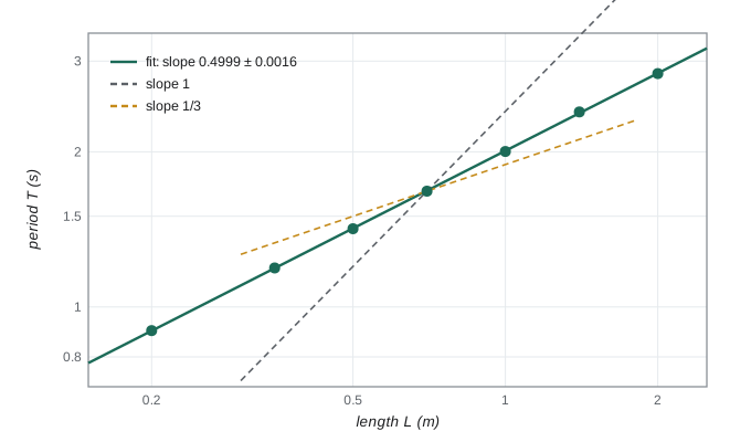
Dimensional analysis tells an experimenter what to plot. If the theory is right, a graph of \(\log T\) against \(\log L\) at fixed amplitude is a straight line of slope one half. Testing the exponent is a sharper test than testing a single value, because many plausible errors would change the slope. It also tells you what is safe to ignore: the mass of the bob does not enter, so changing bobs is a test of the theory, not a variable to control.

Scaling and log-log plots

Power laws are everywhere in physics: the period of a pendulum, the radiated power of a hot body (\(T^4\)), the intensity from a point source (\(r^{-2}\)), the drag on a slow sphere (\(v^1\)) or a fast one (\(v^2\)). A power law \(y = A x^p\) becomes a straight line on a log-log plot, \(\log y = \log A + p\log x\), with slope \(p\). Plotting data this way gives a quick visual test of a power law and a fit gives the exponent with an uncertainty. A curve on the log-log plot means the relation is not a single power law: perhaps two regimes, such as Stokes drag at low speed and quadratic drag at high speed, with a crossover.

Range, spacing and lever arm

Where should the data points go? If you want the slope of a line, spread the points over the widest range you can, because the uncertainty in a fitted slope is inversely proportional to the spread of the independent variable. For points of equal scatter \(\sigma\), the slope uncertainty is \(\sigma/\sqrt{\sum (x_i - \bar{x})^2}\). Seven points crowded between 0.9 m and 1.1 m determine a slope about nine times less well than seven points spread from 0.2 m to 2.0 m. For a power law, space the points evenly in \(\log x\) rather than in \(x\), so that each decade carries equal weight. If you suspect curvature, you need points throughout the range, not only at the ends, or you cannot see it. And always include some points where the theory makes a sharp prediction, such as a threshold or a zero.

How much data do you need?

The precision you need follows from the question. To test whether a slope is one half, you need an uncertainty well below the difference between one half and any competing value. To measure \(g\) well enough to see its variation with latitude, about 5 parts in 1000 between equator and pole, you need better than 1 part in 1000. Once the target is set, the standard error formula \(\sigma_{\bar x} = s/\sqrt{N}\) tells you how many repeats are needed. Because the error falls only as the square root, each extra factor of two in precision costs four times as many measurements. The program shows the arithmetic: if one timing has a scatter of 12 ms, six repeats give 5 ms, but 1 ms needs 144. At some point it is cheaper to improve the method than to repeat it.

import math, random
random.seed(397)
# 1. Dimensional analysis predicts T = C * sqrt(L/g). Test the exponent with a log-log fit.
g = 9.81
lengths = [0.20, 0.35, 0.50, 0.70, 1.00, 1.40, 2.00]
data = [(L, 2*math.pi*math.sqrt(L/g)*(1 + random.gauss(0, 0.004))) for L in lengths]   # 0.4 % timing scatter
X = [math.log(L) for L, T in data]; Y = [math.log(T) for L, T in data]
n = len(X); mx, my = sum(X)/n, sum(Y)/n
Sxx = sum((x - mx)**2 for x in X); Sxy = sum((x - mx)*(y - my) for x, y in zip(X, Y))
slope = Sxy/Sxx; icpt = my - slope*mx
res = [y - (icpt + slope*x) for x, y in zip(X, Y)]
s = math.sqrt(sum(r*r for r in res)/(n - 2))
print(f"log-log slope = {slope:.4f} +/- {s/math.sqrt(Sxx):.4f}  (dimensional analysis: 0.5)")
C = math.exp(icpt)*math.sqrt(g)
print(f"dimensionless constant C = {C:.3f}  (theory 2 pi = {2*math.pi:.3f})")
# 2. How many repeats are needed? The standard error falls as s/sqrt(N).
s1 = 0.012     # scatter of one timing of 20 swings, in seconds
for target in (0.005, 0.002, 0.001):
    N = math.ceil((s1/target)**2)
    print(f"to reach a standard error of {target*1000:.0f} ms with s = {s1*1000:.0f} ms needs N = {N} repeats")
# 3. Choosing the range: the uncertainty in a fitted slope shrinks as the lever arm grows.
for span in ((0.9, 1.1), (0.5, 1.5), (0.2, 2.0)):
    xs = [span[0] + (span[1] - span[0])*i/6 for i in range(7)]
    m = sum(xs)/7; sxx = sum((x - m)**2 for x in xs)
    print(f"7 points from {span[0]} to {span[1]} m: slope uncertainty = {1/math.sqrt(sxx):.2f} x (point scatter)")

log-log slope = 0.4999 +/- 0.0016  (dimensional analysis: 0.5)
dimensionless constant C = 6.294  (theory 2 pi = 6.283)
to reach a standard error of 5 ms with s = 12 ms needs N = 6 repeats
to reach a standard error of 2 ms with s = 12 ms needs N = 36 repeats
to reach a standard error of 1 ms with s = 12 ms needs N = 144 repeats
7 points from 0.9 to 1.1 m: slope uncertainty = 5.67 x (point scatter)
7 points from 0.5 to 1.5 m: slope uncertainty = 1.13 x (point scatter)
7 points from 0.2 to 2.0 m: slope uncertainty = 0.63 x (point scatter)

The fitted exponent, \(0.4999 \pm 0.0016\), agrees with one half to within a tenth of its uncertainty, and the dimensionless constant comes out as 6.294, close to \(2\pi = 6.283\); the small difference is consistent with the 4 parts in 1000 of timing scatter built into the simulated data. The last three lines quantify the lever-arm effect: compressing the range from 0.2 to 2.0 m down to 0.9 to 1.1 m makes the slope nine times less certain for the same number of points.

Pilot experiments and the error budget

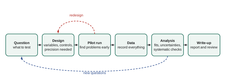
Real apparatus rarely behaves as planned. A pilot run, a quick rough version of the whole experiment, reveals problems while they are cheap to fix: the signal is smaller than expected, a cable picks up mains hum, the sample heats up, the reading drifts. It also gives the first realistic estimate of each source of uncertainty. Write these down in an error budget, a table listing every contribution to the final uncertainty with its estimated size. The budget shows where effort will pay: there is no point buying a better ruler if the timing dominates. In the pendulum experiment, a typical budget might show a length contribution of 1 part in 1000, timing 0.5 parts in 1000 after timing 50 swings, and amplitude bias 2 parts in 1000 unless corrected. The budget makes it obvious that the amplitude correction, not better timing, is the next job.

Blind analysis

Experimenters are human, and humans tend to stop looking for mistakes once they get the answer they expected. Particle physicists and cosmologists now often use blind analysis: the key number is hidden, for example by adding an unknown offset to the data, until all the cuts, corrections and uncertainty estimates have been fixed. Only then is the box opened. A blind analysis cannot remove systematic errors, but it prevents the experimenter's expectations from steering the choices that determine the result. The idea scales down to the teaching lab: decide in advance how you will analyze the data and which points, if any, you will reject, before you see how the answer comes out.