
PHYS-230 · Lesson 3 of 12 · 25 min
Damped and driven oscillations and resonance
Real oscillators lose energy. A swing slows to a stop, a plucked string fades, and the current in a radio circuit dies away unless something keeps feeding it. And real oscillators are pushed: a child is pushed on the swing, wind gusts push a bridge, and an antenna drives the circuit in a receiver. This lesson adds both effects to the harmonic oscillator. Damping turns the oscillation into a decaying one with three distinct regimes. Driving at a frequency \(\omega\) produces a steady response whose amplitude and phase depend sharply on how close \(\omega\) is to the natural frequency, the phenomenon of resonance. One number, the quality factor \(Q\), captures how sharp that resonance is and how slowly the free oscillation decays, and it is the single most useful figure of merit for an oscillator.
The damped oscillator
The simplest model of friction that keeps the equation linear is a force proportional to velocity, \(-b\dot x\), which describes viscous drag at low speed, eddy-current braking and the resistance in an electrical circuit. Newton's law becomes \(m\ddot x + b\dot x + kx = 0\). Dividing by \(m\) and writing \(\gamma = b/m\) and \(\omega_0^2 = k/m\),
Try \(x = e^{st}\) again. The characteristic equation \(s^2 + \gamma s + \omega_0^2 = 0\) has roots
Three cases follow from the sign of the discriminant. If \(\gamma < 2\omega_0\), the system is underdamped: the roots are complex, \(s = -\gamma/2 \pm i\omega_d\) with \(\omega_d = \sqrt{\omega_0^2 - \gamma^2/4}\), and the motion is
an oscillation at a slightly lowered frequency inside an exponentially shrinking envelope. If \(\gamma > 2\omega_0\), the system is overdamped: both roots are real and negative, and \(x(t)\) is a sum of two decaying exponentials that creeps back to equilibrium without oscillating. If \(\gamma = 2\omega_0\) exactly, the system is critically damped: the roots coincide at \(-\omega_0\), and the second independent solution is \(te^{-\omega_0 t}\), so \(x(t) = (C_1 + C_2 t)e^{-\omega_0 t}\). Critical damping returns the system to equilibrium fastest without overshoot, which is why car suspensions, analog meter needles and door closers are designed to be close to it.
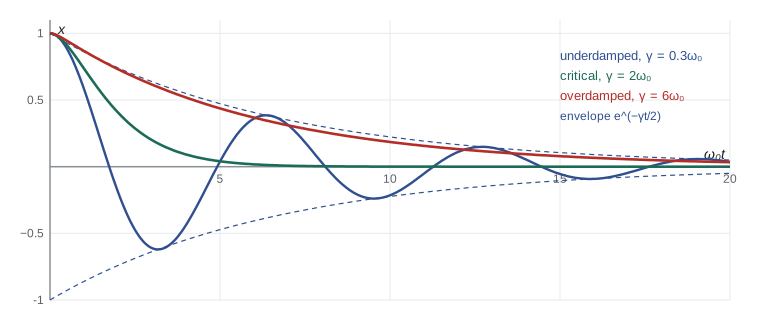
For the overdamped case the slower of the two decay rates is \(\gamma/2 - \sqrt{\gamma^2/4 - \omega_0^2}\), which for heavy damping is approximately \(\omega_0^2/\gamma\). So making the damping heavier makes the return slower, not faster: a door closer filled with very thick oil takes ages to shut. That is the sense in which critical damping is optimal.
Energy loss and the quality factor
The energy \(E = \tfrac12 m\dot x^2 + \tfrac12 kx^2\) now changes at the rate \(dE/dt = m\dot x\ddot x + kx\dot x = -b\dot x^2\), the power dissipated by the drag force. For light damping, average over one cycle: \(\langle \dot x^2 \rangle = E/m\), so \(d\langle E \rangle/dt = -\gamma \langle E \rangle\) and the energy decays as \(e^{-\gamma t}\), twice as fast as the amplitude, as it must since energy goes as amplitude squared. The time \(\tau = 1/\gamma\) is the energy decay time.
The quality factor is defined as
The second form follows because the energy lost in one period \(2\pi/\omega_0\) is \(\gamma E \cdot 2\pi/\omega_0\). A high-\(Q\) oscillator rings for about \(Q/\pi\) cycles before its amplitude falls by a factor \(e\). Another convenient measure is the logarithmic decrement \(\Lambda = \ln(x_n / x_{n+1})\), the natural logarithm of the ratio of successive peaks, which equals \(\gamma T_d / 2 \approx \pi / Q\) for light damping. Measuring two peaks a known number of cycles apart is the standard way to find \(Q\) in the laboratory.
| Oscillator | Typical Q | What it means |
|---|---|---|
| Car suspension | about 0.5 to 1 | near critical damping, little bounce |
| Guitar string | about 1,000 | rings for a few seconds |
| Tuning fork | about 1,000 to 10,000 | a long, pure tone |
| Quartz watch crystal | about 10,000 to 100,000 | very stable frequency |
| Microwave cavity, superconducting | up to about 10 billion | used in particle accelerators |
| Optical cavity of a laser | about a million to a billion | very narrow spectral lines |
Worked problem
Finding Q from a ring-down
A tuning fork at 440 Hz is struck, and its sound amplitude falls to half its initial value in 6.0 s. Find \(\gamma\), \(Q\) and the number of cycles in that time.
Show solution
- The amplitude decays as \(e^{-\gamma t/2}\), so \(e^{-\gamma(6.0)/2} = 0.5\) gives \(\gamma = 2\ln2/6.0 = 0.231\ \mathrm{s^{-1}}\).
- \(\omega_0 = 2\pi(440) = 2765\ \mathrm{rad/s}\), so \(Q = \omega_0/\gamma \approx 1.20\times10^4\).
- In 6.0 s the fork completes \(440 \times 6.0 = 2640\) cycles.
Answer: \(\gamma \approx 0.23\ \mathrm{s^{-1}}\) and \(Q \approx 12{,}000\). The shift of the oscillation frequency from damping, \(\omega_0 - \omega_d \approx \gamma^2/8\omega_0\), is about \(2\times10^{-6}\ \mathrm{rad/s}\), utterly negligible.
The driven oscillator
Now add a sinusoidal driving force \(F_0\cos\omega t\):
The general solution is a particular solution plus the general solution of the undriven equation. The undriven part decays as \(e^{-\gamma t/2}\), so after a few decay times only the particular solution, the steady state, remains. To find it, replace the drive by \((F_0/m)e^{i\omega t}\) and look for \(x = \tilde A e^{i\omega t}\), taking the real part at the end. Each time derivative brings down \(i\omega\), so
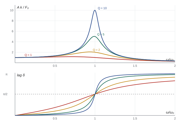
The modulus and argument of \(\tilde A\) give the amplitude and the phase lag \(\delta\) of the response behind the drive, \(x = A\cos(\omega t - \delta)\):
Three regimes are worth knowing. Far below resonance, \(\omega \ll \omega_0\), the amplitude is \(F_0/k\), the static deflection, and the response is in phase with the drive: the spring dominates. Far above, \(\omega \gg \omega_0\), the amplitude falls as \(F_0/m\omega^2\) and the response is half a cycle behind: inertia dominates, and the mass moves opposite the force. At \(\omega = \omega_0\) the phase lag is exactly a quarter cycle, the velocity is in phase with the force, and the amplitude is \(F_0/(m\gamma\omega_0) = Q F_0/k\), larger than the static deflection by the factor \(Q\). The amplitude itself peaks slightly below \(\omega_0\), at \(\omega_r = \sqrt{\omega_0^2 - \gamma^2/2}\), a shift that is negligible for high \(Q\).
Power and bandwidth
The average power delivered by the drive is the average of force times velocity. With \(\dot x = -\omega A\sin(\omega t - \delta)\), only the part of the velocity in phase with \(\cos\omega t\) contributes, and a short calculation gives
In steady state this equals the power dissipated by damping, \(b\langle\dot x^2\rangle\). It peaks exactly at \(\omega_0\), at the value \(F_0^2/2m\gamma\). Near resonance, writing \(\omega_0^2 - \omega^2 \approx 2\omega_0(\omega_0 - \omega)\) turns the power curve into the Lorentzian \(\langle P\rangle \propto 1/[(\omega - \omega_0)^2 + (\gamma/2)^2]\), whose full width at half maximum is \(\Delta\omega = \gamma\). Hence
This is the second meaning of \(Q\): the ratio of the resonant frequency to the width of the resonance. A radio receiver must select one station among neighbors spaced about 10 kHz apart near 1 MHz, so its tuned circuit needs \(Q\) of order 100. The two meanings of \(Q\) are linked by a deep fact: a resonance that is sharp in frequency must ring for a long time, because a narrow band of frequencies can only be built from a long wave train. Lesson 7 makes this precise with the Fourier transform.
Worked problem
A tuned circuit
A series RLC circuit has \(L = 250\ \mathrm{\mu H}\), \(C = 100\ \mathrm{pF}\) and \(R = 10\ \Omega\). Find its resonant frequency, its \(Q\) and its bandwidth.
Show solution
- The circuit equation \(L\ddot q + R\dot q + q/C = V(t)\) matches the oscillator with \(\gamma = R/L\) and \(\omega_0 = 1/\sqrt{LC}\).
- \(\omega_0 = 1/\sqrt{250\times10^{-6}\cdot100\times10^{-12}} = 6.32\times10^6\ \mathrm{rad/s}\), so \(f_0 = 1.01\ \mathrm{MHz}\).
- \(\gamma = 10/250\times10^{-6} = 4.0\times10^4\ \mathrm{s^{-1}}\), so \(Q = \omega_0/\gamma \approx 158\).
- The bandwidth is \(\Delta f = f_0/Q \approx 6.4\ \mathrm{kHz}\).
Answer: \(f_0 \approx 1.01\ \mathrm{MHz}\), \(Q \approx 158\), bandwidth about 6.4 kHz: enough to separate AM stations 10 kHz apart.
Transients and beats
When the drive is switched on, the full solution is the steady state plus a decaying free oscillation at \(\omega_d\) chosen to match the initial conditions. Before the transient dies, the two frequencies \(\omega\) and \(\omega_d\) beat against each other: the amplitude swells and shrinks at the difference frequency \(|\omega - \omega_d|\). For a high-\(Q\) system driven exactly at resonance and starting from rest, the amplitude grows as \(A_{\text{ss}}(1 - e^{-\gamma t/2})\), approaching its steady value over a time of order \(2Q/\omega_0\). This is why it takes many pushes to build up a large swing, and why a sudden short gust cannot excite a high-\(Q\) structure to its full resonant amplitude.
Resonance in engineering
Resonance is useful in clocks, filters, musical instruments, MRI and lasers, and dangerous in structures and machinery. The collapse of the Tacoma Narrows Bridge in 1940 is often cited as resonance, but the mechanism was aeroelastic flutter: the twisting deck and the wind exchanged energy so that the effective damping became negative and the oscillation grew without an external periodic force at the bridge frequency. Ordinary forced resonance does trouble footbridges: when the Millennium Bridge in London opened in 2000, walkers fell into step with a sideways sway near 1 Hz and the bridge closed for two years while dampers were fitted. Tall buildings use tuned mass dampers, large masses on springs tuned near the building's frequency so that they absorb its motion; the one in Taipei 101 is a sphere of about 660 metric tons. Rotating machinery is run through its critical speeds quickly so that resonance never has time to build up.
Computing resonance curves
The program tabulates the steady-state amplitude and phase for \(Q = 10\), checks numerically that the half-power width of the power curve equals \(\gamma\), and then integrates the driven equation from rest at resonance with velocity Verlet to watch the amplitude approach its steady value.
import math, cmath

w0, Q = 1.0, 10.0
g = w0 / Q                       # gamma
F_over_m = 1.0

def response(w):
    A = F_over_m / complex(w0*w0 - w*w, g*w)
    return abs(A), -cmath.phase(A)          # amplitude and phase lag

print(" w/w0   A*k/F0   lag/pi")
for w in (0.2, 0.5, 0.8, 0.9, 0.95, 1.0, 1.05, 1.1, 1.5, 2.0):
    A, d = response(w)
    print(f"{w:5.2f}  {A*w0*w0:7.3f}  {d/math.pi:6.3f}")

# half-power width of <P> = (F^2/2m) g w^2 / ((w0^2-w^2)^2 + g^2 w^2)
P = lambda w: g*w*w / ((w0*w0 - w*w)**2 + (g*w)**2)
Pmax = P(w0)
def cross(lo, hi):
    for _ in range(80):
        mid = (lo + hi) / 2
        if (P(mid) - Pmax/2) * (P(lo) - Pmax/2) <= 0: hi = mid
        else: lo = mid
    return (lo + hi) / 2
wl, wh = cross(0.5, 1.0), cross(1.0, 1.5)
print(f"\nhalf-power points {wl:.5f}, {wh:.5f}; width {wh-wl:.5f}; gamma = {g:.5f}")
print(f"amplitude peak at sqrt(w0^2 - g^2/2) = {math.sqrt(w0*w0 - g*g/2):.5f}")

# switch on the drive at resonance from rest and integrate
x, v, t, dt = 0.0, 0.0, 0.0, 0.001
acc = lambda x, v, t: F_over_m*math.cos(w0*t) - g*v - w0*w0*x
A_ss = Q / (w0*w0)
peak, next_report = 0.0, 10.0
while t < 60.0:
    a = acc(x, v, t)
    v_half = v + 0.5*a*dt
    x = x + v_half*dt
    t += dt
    v = v_half + 0.5*acc(x, v_half, t)*dt
    peak = max(peak, abs(x))
    if t >= next_report:
        print(f"t = {t:4.0f}: largest |x| so far {peak:6.3f}, predicted envelope {A_ss*(1-math.exp(-g*t/2)):6.3f}")
next_report += 10.0w/w0 A*k/F0 lag/pi 0.20 1.041 0.007 0.50 1.330 0.021 0.80 2.712 0.070 0.90 4.757 0.141 0.95 7.346 0.246 1.00 10.000 0.500 1.05 6.815 0.746 1.10 4.218 0.846 1.50 0.794 0.962 2.00 0.333 0.979 half-power points 0.95125, 1.05125; width 0.10000; gamma = 0.10000 amplitude peak at sqrt(w0^2 - g^2/2) = 0.99750 t = 10: largest |x| so far 3.251, predicted envelope 3.935 t = 20: largest |x| so far 5.806, predicted envelope 6.321 t = 30: largest |x| so far 7.750, predicted envelope 7.769 t = 40: largest |x| so far 8.596, predicted envelope 8.647 t = 50: largest |x| so far 9.124, predicted envelope 9.179 t = 60: largest |x| so far 9.454, predicted envelope 9.502
The table shows the amplitude rising from about 1.04 at \(\omega = 0.2\omega_0\) to exactly 10 at resonance, where the lag is half of \(\pi\), and falling to 0.33 at \(2\omega_0\) with a lag approaching \(\pi\). The half-power points sit close to \(\omega_0 \mp \gamma/2\), at 0.951 and 1.051, and their separation is exactly \(\gamma = 0.1\); for this power curve the width equals \(\gamma\) at any \(Q\), not only approximately. The simulation shows the amplitude creeping up toward \(Q F_0/k = 10\) over the time scale \(2/\gamma = 20\), tracking the envelope \(1 - e^{-\gamma t/2}\).
Common mistakes
MistakeAssuming heavier damping always returns a system to equilibrium faster.
InsteadBeyond critical damping the return slows, with rate about \(\omega_0^2/\gamma\).
MistakeSaying the amplitude of a driven oscillator peaks exactly at \(\omega_0\).
InsteadThe power peaks at \(\omega_0\); the displacement amplitude peaks at \(\sqrt{\omega_0^2 - \gamma^2/2}\), slightly lower.
MistakeForgetting the phase lag of a driven oscillator.
InsteadThe response lags by \(\delta\), from 0 well below resonance through \(\pi/2\) at resonance to nearly \(\pi\) well above.
MistakeIncluding the transient when asked for the steady state, or ignoring it when asked about the start.
InsteadThe transient decays as \(e^{-\gamma t/2}\); it matters for times shorter than a few \(2/\gamma\).
MistakeCalling the Tacoma Narrows collapse simple forced resonance.
InsteadIt was aeroelastic flutter, a self-excited oscillation with negative effective damping.
Summary and key terms
- \(\ddot x + \gamma\dot x + \omega_0^2x = 0\) is underdamped for \(\gamma < 2\omega_0\), critically damped at \(\gamma = 2\omega_0\) and overdamped above.
- Underdamped motion is \(Ae^{-\gamma t/2}\cos(\omega_d t + \phi)\) with \(\omega_d = \sqrt{\omega_0^2 - \gamma^2/4}\); energy decays as \(e^{-\gamma t}\).
- \(Q = \omega_0/\gamma = 2\pi\) times stored energy over energy lost per cycle \(= \omega_0/\Delta\omega\).
- The steady-state complex amplitude is \((F_0/m)/(\omega_0^2 - \omega^2 + i\gamma\omega)\); the lag is \(\pi/2\) at resonance, where the amplitude is \(Q\) times the static deflection.
- Drive power is Lorentzian near resonance with full width \(\gamma\); the transient beats and decays over a time of order \(2Q/\omega_0\).
- damping rate
- The coefficient gamma, equal to b over m, in the damped oscillator equation.
- critical damping
- The damping gamma equal to 2 omega zero, the fastest return without overshoot.
- quality factor
- Q, the ratio of natural frequency to damping rate, or of resonant frequency to bandwidth.
- logarithmic decrement
- The natural logarithm of the ratio of successive peaks of a decaying oscillation.
- steady state
- The part of a driven response that remains after the transient has decayed.
- Lorentzian
- The resonance line shape 1 over ((omega minus omega zero) squared plus (gamma over 2) squared).
Practice problems
Work each problem on paper first, then reveal the answer to check.
A 1.5 kg mass on a 600 N/m spring has damping \(b = 3.0\ \mathrm{kg/s}\). Find \(\omega_0\), \(\gamma\), \(Q\) and the critical value of \(b\).
Show answer
\(\omega_0 = 20\ \mathrm{rad/s}\), \(\gamma = 2.0\ \mathrm{s^{-1}}\), \(Q = 10\); critical damping needs \(b = 2m\omega_0 = 60\ \mathrm{kg/s}\).
Successive peaks of a decaying oscillation are 8.0 mm and 7.2 mm. Estimate \(Q\).
Show answer
\(\Lambda = \ln(8.0/7.2) = 0.105\), so \(Q \approx \pi/\Lambda \approx 30\).
For the oscillator in problem 1 driven by \(F_0 = 2.0\ \mathrm{N}\), find the steady amplitude at \(\omega = 10\), 20 and 40 rad/s.
Show answer
\(A = (F_0/m)/\sqrt{(\omega_0^2 - \omega^2)^2 + \gamma^2\omega^2}\): 4.4 mm, 33 mm, 1.1 mm.
Show that at resonance the velocity of a driven oscillator is in phase with the force.
Show answer
At \(\omega = \omega_0\), \(\delta = \pi/2\), so \(x = A\sin\omega t\) and \(\dot x = A\omega\cos\omega t\), in phase with \(F_0\cos\omega t\).
A 100 MHz FM receiver must pass about 200 kHz. What \(Q\) is needed?
Show answer
\(Q = f_0/\Delta f = 10^8/2\times10^5 = 500\).
A heavily overdamped system has \(\omega_0 = 5\ \mathrm{rad/s}\) and \(\gamma = 50\ \mathrm{s^{-1}}\). Estimate its slow return time.
Show answer
Slow rate \(\approx \omega_0^2/\gamma = 0.5\ \mathrm{s^{-1}}\), so the time constant is about 2 s, ten times longer than critical damping's \(1/\omega_0 = 0.2\ \mathrm{s}\).
Lesson quiz · 5 questions
Score 60% or more to complete this lesson.
Create a free account to save your progress, take quizzes and earn a certificate.