Plume modeling and pressure management

The permit application would rest on one map more than any other: the predicted extent of the CO₂ plume and of the pressure increase it causes, now and long after injection stops. “The plume is what people picture,” Farid told Ethan. “The pressure is what the regulator worries about. It travels tens of kilometers, much farther than the CO₂, and it is the pressure that pushes brine up an old well or onto a fault.” Before building the full simulation model, Ethan used analytical solutions to get a feel for both, check the well layout and set up the questions the simulation had to answer.

Two fronts that move at different speeds

Injection creates two disturbances. The CO₂ plume is a volume of rock containing free CO₂, growing roughly with the injected volume; its edge moves at speeds of meters to hundreds of meters a year. The pressure front is a diffusive disturbance in the brine, traveling at a rate set by the hydraulic diffusivity k/(φμc_t), which for permeable rock is kilometers in months. After 25 years the plume of a large project may be a few kilometers across while measurable pressure extends tens to over a hundred kilometers. The area of review that regulators require is usually set by pressure, not by the plume.

The plume: a sharp-interface model

Nordbotten, Celia and Bachu (2005) derived a simple estimate of the plume shape for injection into a confined, horizontal formation, assuming a sharp interface between CO₂ and brine and that viscous forces dominate buoyancy near the well. The plume is thickest at the well and thins outward; its maximum radius at the top of the formation is:

V(t) is the injected volume at reservoir conditions, and λ the mobility ratio of CO₂ to brine. A high mobility ratio makes the plume thin and wide, because CO₂ travels preferentially along the top. In reality, buoyancy makes the plume even more top-heavy, layering in the formation splits it into several tongues under thin shale breaks, as at Sleipner, and dip sends it up-slope. The analytical estimate is still a useful first check and a way to test the simulation model.

The pressure: the Theis solution

Pressure buildup in the brine beyond the plume follows the line-source solution familiar from well testing:

Here q is the reservoir volume rate and E₁ the exponential integral. Buildup from several wells is found by superposition: add the buildup each well causes at the point of interest. At the injection well, the pressure also includes the steady-state drop across the CO₂-filled region near the well, which is small because CO₂ is mobile. The code below combines these to estimate the pressure at the middle well of the hub's four-well line, where interference is worst.

# CO2 plume radius (Nordbotten-Celia sharp interface) and pressure buildup (Theis line source with superposition)
# for the hub's injection wells over 25 years. Illustrative single-layer, homogeneous model.
import math
SI = False     # True: Canadian hub (Basal Cambrian), metric; False: US hub (Frio), US units

if SI: P = dict(h=45.0, phi=0.16, k=250, mu_w=7.5e-4, mu_c=6.0e-5, rho_c=704.0, ct=1.2e-9, krc=0.35, p0=20.5e6, plim=33.2e6, wells=4, spacing=4000.0)
else:  P = dict(h=45.7, phi=0.26, k=300, mu_w=4.5e-4, mu_c=5.0e-5, rho_c=573.0, ct=1.2e-9, krc=0.35, p0=18.2e6, plim=26.1e6, wells=4, spacing=4000.0)
YEAR = 3.156e7; RW = 0.10
k = P['k'] * 9.869e-16                       # mD to m2
q_mass = 3.0e9 / YEAR / P['wells']           # kg/s per well (3.0 Mt/yr hub)
q = q_mass / P['rho_c']                      # reservoir m3/s per well
lam = (P['krc'] / P['mu_c']) / (1 / P['mu_w'])   # mobility ratio CO2/brine

def E1(u):                                   # exponential integral, series for small u, continued fraction otherwise
    if u < 1:
        s, term, n = -0.5772156649 - math.log(u), 1.0, 1
        while True:
            term *= -u / n; add = -term / n; s += add; n += 1
            if abs(add) < 1e-14: return s
    f = u
    for n in range(40, 0, -1): f = u + n / (1 + n / f)
    return math.exp(-u) / f

def theis(r, t):
    return q * P['mu_w'] / (4 * math.pi * k * P['h']) * E1(r * r * P['phi'] * P['mu_w'] * P['ct'] / (4 * k * t))

def plume(t):
    V = q * t
    return math.sqrt(lam * V / (math.pi * P['phi'] * P['h']))

def well_dp(t, n_wells):
    rp = plume(t)
    dp_co2 = q * P['mu_c'] / (2 * math.pi * k * P['krc'] * P['h']) * math.log(rp / RW)   # CO2 zone, steady
    dp_own = theis(rp, t)                                                              # brine beyond the plume
    # neighbors on a line at the given spacing; the worst well is in the middle
    others = sum(theis(abs(j - n_wells // 2) * P['spacing'], t) for j in range(n_wells) if j != n_wells // 2)
    return dp_co2, dp_own, others

conv_r = (lambda m: f"{m:,.0f} m") if SI else (lambda m: f"{m * 3.281:,.0f} ft")
conv_p = (lambda pa: f"{pa / 1e6:.1f} MPa") if SI else (lambda pa: f"{pa / 6894.8:,.0f} psi")
print(f"Per well: {q_mass * YEAR / 1e9:.2f} Mt/yr, {q:.4f} reservoir m3/s; mobility ratio CO2/brine {lam:.1f}")
print(f"Allowed buildup at the well: {conv_p(P['plim'] - P['p0'])}")
print(" year   plume radius   CO2 zone   own brine   neighbors   total")
for yr in (1, 5, 10, 15, 25):
    t = yr * YEAR; a, b, c = well_dp(t, P['wells'])
    flag = '' if a + b + c <= P['plim'] - P['p0'] else '  over limit'
    print(f"{yr:5d}   {conv_r(plume(t)):>12s}   {conv_p(a):>8s}   {conv_p(b):>9s}   {conv_p(c):>10s}   {conv_p(a + b + c):>7s}{flag}")
# pressure management option: one brine producer per two injectors cuts the far-field buildup roughly in proportion to net voidage
t = 25 * YEAR; a, b, c = well_dp(t, P['wells'])
for frac in (0.0, 0.25, 0.5):
    print(f"Brine extraction at {frac:.0%} of injected volume: total buildup about {conv_p(a + (b + c) * (1 - frac))} after 25 years")
r_inv = math.sqrt(4 * k * t / (P['phi'] * P['mu_w'] * P['ct']))
print(f"Radius of investigation after 25 years, sqrt(4kt/(phi mu ct)): {conv_r(r_inv)}")
# if faults or a neighboring hub confined the hub to its own tenure, the formation behaves like a closed box
area = 800e6 if SI else 600e6
pore = area * P['h'] * P['phi']; V = 3.0e9 * 25 / P['rho_c']
print(f"Closed-box check: {V / 1e6:,.0f} million m3 injected into {pore / 1e9:.2f} billion m3 of pore space "
      f"raises the average pressure by {conv_p(V / (pore * P['ct']))}, against {conv_p(P['plim'] - P['p0'])} allowed.")

Per well: 0.75 Mt/yr, 0.0415 reservoir m3/s; mobility ratio CO2/brine 3.1
Allowed buildup at the well: 1,146 psi
 year   plume radius   CO2 zone   own brine   neighbors   total
    1       1,090 ft     82 psi     115 psi       90 psi   287 psi
    5       2,438 ft     90 psi     115 psi      163 psi   368 psi
   10       3,448 ft     94 psi     115 psi      195 psi   404 psi
   15       4,223 ft     96 psi     115 psi      214 psi   425 psi
   25       5,452 ft     98 psi     115 psi      239 psi   452 psi
Brine extraction at 0% of injected volume: total buildup about 452 psi after 25 years
Brine extraction at 25% of injected volume: total buildup about 363 psi after 25 years
Brine extraction at 50% of injected volume: total buildup about 275 psi after 25 years
Radius of investigation after 25 years, sqrt(4kt/(phi mu ct)): 267,663 ft
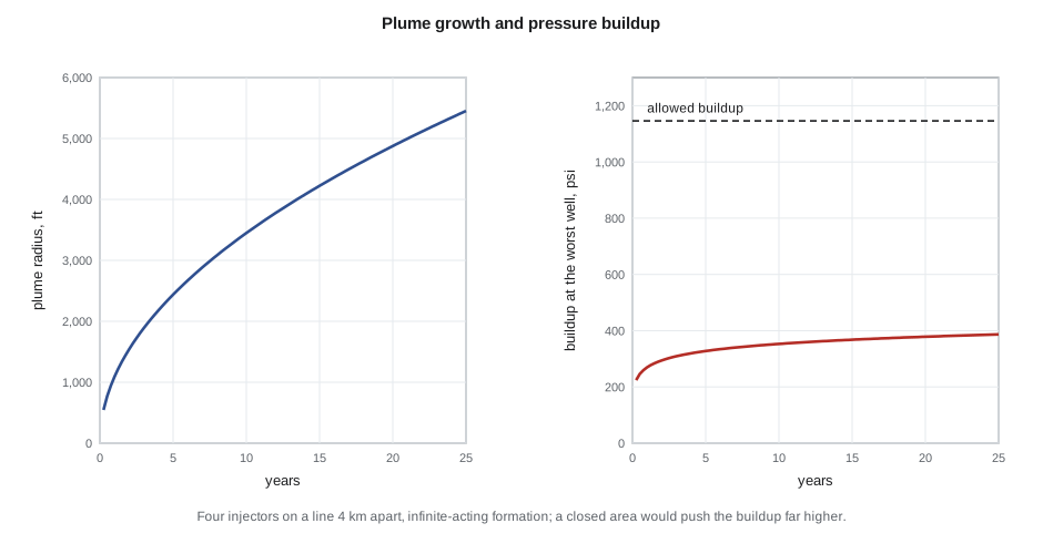
Closed-box check: 131 million m3 injected into 7.13 billion m3 of pore space raises the average pressure by 2,219 psi, against 1,146 psi allowed.

The plume around each well reaches about 5,500 ft in radius after 25 years. Pressure at the worst well rises quickly in the first year, then slowly, reaching about 450 psi against an allowed 1,146 psi; about half of it comes from the neighboring wells. That is comfortable if the formation is effectively infinite. The closed-box check shows the other extreme: if the hub's own area could not shed pressure, the average rise would exceed the limit before 25 years. The truth lies between, and depends on the regional extent and permeability of the Frio and on what other projects inject into it. Several permitted and proposed Class VI projects target the same Gulf Coast sands, so the RRC expects each project's model to account for its neighbors.

The area of review

The area of review is the region in which the project must find and evaluate every well and pathway that could let CO₂ or brine escape from the storage complex. One common way to define it is the area where the pressure increase is enough to push formation brine up an open wellbore to the base of the lowest underground source of drinking water. If the formation and the drinking water aquifer start in hydrostatic equilibrium, the critical pressure increase is:

where p_u is the pressure at the base of the drinking water zone at depth z_u, ρ_b the density of the formation brine, z_i the depth of the injection zone and p_i its initial pressure. For a brine much denser than fresh water, Δp_c is relatively large; for a formation that is overpressured or whose brine is fresh, it can be near zero, making the area of review very large.

EPA's Class VI rules require the area of review to be delineated by computational modeling of both the plume and the pressure front, and re-evaluated at least every five years with monitoring data.

Numerical simulation

The permit-quality model is a numerical reservoir simulation. It solves for two phases, CO₂-rich and brine-rich, with CO₂ dissolving in brine and water evaporating into CO₂, using either a compositional simulator or a modified black-oil formulation in which CO₂ plays the role of gas and dissolved CO₂ the role of solution gas. The grid must be fine vertically under the seal, where the plume is thin, often a meter or less, while extending tens of kilometers laterally to capture the pressure; local grid refinement or vertical-equilibrium models, which assume buoyant segregation in each column, manage the cost. Geomechanical coupling estimates the stresses on faults and the seal, and surface uplift. The inputs carry the uncertainties of characterization, so models are run as ensembles, and the results are given as ranges.

Once injection starts, the model is history matched to monitoring data: injection pressures and falloff tests, pressure in monitoring wells, the plume's footprint in repeat seismic, and saturation logs. Sleipner's plume, imaged in seismic since 1999, spread under nine thin shale layers that no pre-injection model predicted, and matching it improved understanding of buoyant flow in layered sands. At In Salah in Algeria, satellite radar measured surface uplift of a few millimeters a year above the injectors, revealing that injection pressure had opened a fracture zone above the reservoir; injection was reduced and later suspended. Both projects show why models are updated with data and why the permit expects it.

Pressure management

When pressure is the constraint, there are several ways to manage it. Spreading wells and injecting in several zones lowers interference. Allocating rate across wells, more where the rock is better and less near faults, keeps every well below its limit. Extracting brine from the formation, a few kilometers from the injectors, creates space and lowers pressure across the area; the code shows that producing brine equal to half the injected volume cuts the buildup at the wells by about 40 percent. The produced brine must be disposed of, often into a shallower saline zone, or used, and this adds cost and wells. Brine extraction can also steer the plume. Ethan proposed keeping it as a contingency: a reserved location and a design that could add a brine producer if monitoring showed pressure rising faster than predicted.

Pressure also governs induced seismicity. Keeping the pore pressure increase on each mapped fault below the level that would bring it to slip, with a margin, is part of the injection pressure limit. A traffic-light protocol, used at several projects, sets thresholds of microseismic magnitude or frequency at which injection is reviewed, reduced or stopped.