Storage capacity and injectivity

Lena's question was blunt. “Seventy-five million metric tons over twenty-five years, three million a year. Can the hub area take it, and how many wells does it need?” Ethan knew the answer had two parts that are easy to confuse. Capacity is how much CO₂ the formation can hold; injectivity is how fast wells can put it there. A formation can have enormous capacity and still be a poor site because each well takes only a little CO₂ before pressure reaches its limit, and a highly permeable formation can take CO₂ quickly but fill its legal boundary in a decade. The study had to show both, with ranges.

How capacity is classified

Storage estimates are described with a resource pyramid similar to the petroleum one. Theoretical capacity is the whole pore volume that could physically hold CO₂. Effective capacity applies geological and engineering limits, such as how much of the pore volume a plume can actually contact. Practical capacity adds economic, regulatory and infrastructure limits. Matched capacity pairs storage with real sources and pipelines. The Society of Petroleum Engineers' Storage Resources Management System (SRMS), published in 2017, applies the familiar reserves logic to storage: a project with a defined development plan, permits and commercial commitment can book capacity, which is classified by maturity and uncertainty as low, best and high estimates, like proved, probable and possible reserves.

The efficiency-factor method

For saline formations at the regional and screening stage, the US Department of Energy method is the most widely used. It multiplies the bulk pore volume of the formation by the CO₂ density and a storage efficiency factor:

Here A is the area, h_g the gross thickness, φ_tot the total porosity, ρ_CO₂ the CO₂ density at reservoir conditions and E the efficiency factor. E combines the fractions of the area and thickness that are suitable, the fraction of porosity that is effective, and the displacement efficiencies: how much of the pore volume within the plume's reach CO₂ actually contacts, given buoyancy, heterogeneity and viscous fingering, and how much of each contacted pore it fills, given residual brine. From Monte Carlo analysis of those factors, the DOE gives formation-scale values for clastic formations of about 0.5 percent at P10, 2.0 percent at P50 and 5.5 percent at P90, and somewhat different values for carbonates. If the net thickness and effective porosity are known, higher site-specific factors apply. The point of the method is not precision but honesty about the range: a P10 to P90 spread of a factor of ten is typical before any injection data exist.

# Storage capacity of the hub area (DOE efficiency-factor method and a closed-volume pressure limit)
# and injectivity: how many wells the hub needs.
import math
SI = False     # True: Canadian hub (Basal Cambrian), metric; False: US hub (Frio), US units

if SI: P = dict(area_km2=800, h=45.0, phi=0.16, rho=704.0, ct=1.2e-9, dp=12.7e6, k=250, mu_c=6.0e-5, krc=0.35, tubing=1.0)
else:  P = dict(area_km2=600, h=45.7, phi=0.26, rho=573.0, ct=1.2e-9, dp=7.9e6, k=300, mu_c=5.0e-5, krc=0.35, tubing=1.0)
need = 3.0 * 25                               # Mt over the project life
A = P['area_km2'] * 1e6
pore = A * P['h'] * P['phi']
if SI: print(f"Area {P['area_km2']} km2, net {P['h']:.0f} m, porosity {P['phi']:.2f}: pore volume {pore / 1e9:.2f} billion m3")
else:  print(f"Area {P['area_km2'] / 2.59:.0f} mi2, net {P['h'] * 3.281:.0f} ft, porosity {P['phi']:.2f}: pore volume {pore * 6.2898 / 1e9:.1f} billion bbl")
print(f"CO2 density at reservoir conditions {P['rho']:.0f} kg/m3 ({P['rho'] / 16.0185:.1f} lb/ft3)")
print("DOE efficiency factors for clastic saline formations (formation scale):")
for lab, E in (("P10", 0.0051), ("P50", 0.020), ("P90", 0.055)):
    G = pore * P['rho'] * E / 1e9
    print(f"  {lab}: E = {E:.2%}  capacity {G:6.0f} Mt   {'covers' if G >= need else 'short of'} the {need:.0f} Mt plan")
closed = pore * P['ct'] * P['dp'] * P['rho'] / 1e9
lab = f"{P['dp'] / 1e6:.1f} MPa" if SI else f"{P['dp'] / 6894.8:,.0f} psi"
print(f"Closed-volume limit (pressure rise {lab}, total compressibility {P['ct']:.1e} 1/Pa): {closed:.0f} Mt")

# injectivity: steady radial flow of CO2 with endpoint relative permeability, drawdown budget at the wellbore
k = P['k'] * 9.869e-16
def rate(dp_well, re=1000.0, rw=0.1, skin=2.0):
    qv = 2 * math.pi * k * P['krc'] * P['h'] * dp_well / (P['mu_c'] * (math.log(re / rw) + skin))
    return qv * P['rho'] * 3.156e7 / 1e9          # Mt/yr
print("\nInjectivity per well (Mt/yr) for near-well pressure budgets:")
for dpw in (1e6, 2e6, 3e6):
    lab = f"{dpw / 1e6:.0f} MPa" if SI else f"{dpw / 6894.8:,.0f} psi"
    print(f"  {lab:>8s}: reservoir allows {rate(dpw):.2f} Mt/yr; tubing and wellhead limit {P['tubing']:.1f} Mt/yr")
per = min(rate(2e6), P['tubing'])
n = math.ceil(3.0 / per)
print(f"Wells for 3.0 Mt/yr at {per:.2f} Mt/yr each: {n}, plus one spare for workovers = {n + 1}")

Area 232 mi2, net 150 ft, porosity 0.26: pore volume 44.8 billion bbl
CO2 density at reservoir conditions 573 kg/m3 (35.8 lb/ft3)
DOE efficiency factors for clastic saline formations (formation scale):
  P10: E = 0.51%  capacity     21 Mt   short of the 75 Mt plan
  P50: E = 2.00%  capacity     82 Mt   covers the 75 Mt plan
  P90: E = 5.50%  capacity    225 Mt   covers the 75 Mt plan
Closed-volume limit (pressure rise 1,146 psi, total compressibility 1.2e-09 1/Pa): 39 Mt

Injectivity per well (Mt/yr) for near-well pressure budgets:
   145 psi: reservoir allows 0.96 Mt/yr; tubing and wellhead limit 1.0 Mt/yr
   290 psi: reservoir allows 1.92 Mt/yr; tubing and wellhead limit 1.0 Mt/yr
   435 psi: reservoir allows 2.88 Mt/yr; tubing and wellhead limit 1.0 Mt/yr
Wells for 3.0 Mt/yr at 1.00 Mt/yr each: 3, plus one spare for workovers = 4

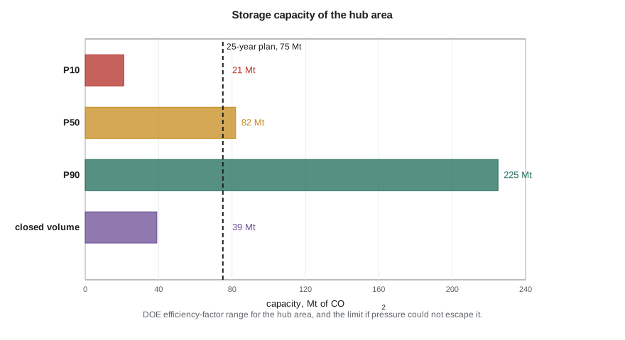
The 232 square mile (600 km²) hub area, with 150 ft of net sand at 26 percent porosity, has about 45 billion barrels (7.1 billion m³) of pore volume. At the P50 efficiency, it holds about 82 million metric tons, just above the plan; at P10 it holds only 21 million, and at P90 about 225 million. Ethan's conclusion was that the area was probably adequate but not certainly, and that the test well and injection test should be planned to narrow the range before any commitment. He also noted that the efficiency factor already includes buoyancy and sweep; using a site simulation instead would give a more defensible number for the permit.

Pressure-limited capacity

The efficiency method assumes the formation is open: the brine displaced by CO₂ moves away, and pressure dissipates into the wider aquifer. If the storage area is closed, by sealing faults, pinch-outs or neighboring projects that raise pressure too, the CO₂ can fit only by compressing the brine and the rock. The capacity is then the injected volume that raises the average pressure to the allowed limit:

With a total compressibility c_t of about 1.2 × 10⁻⁹ Pa⁻¹ and an allowed rise of 7.9 MPa (1,146 psi), the closed-volume capacity is 39 million metric tons, short of the plan. In practice the Frio extends far beyond the hub area, so it is not closed, but neighboring hubs injecting into the same formation would share its pressure capacity. Several Class VI applications in the same Gulf Coast formations have raised the same issue, and pressure interaction between projects is part of each area of review. Lesson 9 calculates the pressure in time and space; the lesson here is that pressure, not pore volume, often limits storage.

Injectivity

Injectivity is the rate a well can inject for a given pressure above the formation pressure. For steady radial flow of CO₂ near the well, Darcy's law gives:

Because CO₂ is about ten times less viscous than brine, its mobility near the well is high even with a reduced relative permeability, so injectivity is usually better than a water injection test suggests. The pressure budget at the well is shared between the near-well flow of CO₂, the pressure buildup in the brine beyond the plume and interference from other wells (Lesson 9). With 300 mD rock and 150 ft of sand, the code shows that a 290 psi near-well drawdown would allow well over a million metric tons a year per well. In practice, the tubing, wellhead equipment and the wish to spread CO₂ over a larger area limited the design rate to 1.0 million metric tons a year per well, so the hub needs three injectors plus one spare for workovers. Gulf Coast storage projects have generally planned for similar rates per well in the Frio and Miocene sands.

Dynamic capacity: rate and time together

Static estimates say how much CO₂ fits; they do not say how fast it can go in. Dynamic capacity combines the two: the total that can be injected over the project life at the planned rate without exceeding the pressure limit anywhere, given the wells, their spacing and the formation's boundaries. It is always less than or equal to the static estimate, and it depends on decisions the engineers control. Spreading wells over a larger area lowers the pressure interference between them; injecting at a steady rate rather than in surges keeps buildup down; and extracting brine from the formation, discussed in Lesson 9, can create room where pressure is the constraint. For the hub, Ethan proposed four well locations on a line about 2.5 miles apart along the strike of the formation, so that their pressure fronts would overlap only after several years, and a fifth location reserved for a future brine producer. The simulation model would test that layout against the full range of capacity and permeability from the test well before the permit application.

Thermal and geochemical effects at the well

Two effects can change injectivity with time. Cold injection cools the rock around the well, reducing the stress there and potentially opening thermal fractures; this can increase injectivity, but fractures that grow into the seal must be avoided, so the design checks the cooled zone's stresses. And dry CO₂ evaporates brine near the well, which in very saline formations can precipitate salt in the pores and reduce permeability, a problem seen in some projects; periodic fresh water injection can redissolve it. Conversely, carbonic acid can dissolve carbonate cement near the well and improve injectivity. Well testing during operations, with falloff tests and continuous pressure monitoring, tracks these changes.

Well design for CO₂

Injection wells for CO₂ are designed for a corrosive fluid if water is ever present. Tubing is often 13 percent chromium steel or carbon steel with a corrosion-resistant lining, the packer and wellhead use CO₂-compatible elastomers, which can blister when dense CO₂ decompresses, and the cement across the seal is a CO₂-resistant blend or a conventional cement placed with great care, since a good bond across the caprock is the main defense against leakage along the well. The annulus is filled with inhibited fluid and its pressure is monitored continuously; a rising annulus pressure is the first sign of a tubing or packer leak. EPA's Class VI rules specify construction, testing and monitoring for CO₂ injection wells, including corrosion-resistant materials and continuous annulus monitoring.

The wellhead pressure of a CO₂ injector is lower than for a gas injector at the same bottomhole pressure, because the dense column in the tubing weighs nearly as much as a water column. At 6,000 ft, a column of CO₂ at about 50 lb/ft³ adds about 2,100 psi of head, so a bottomhole pressure of 2,900 psia needs a wellhead pressure of only about 900 to 1,100 psia, after friction. That is close to the vapor pressure, and if the wellhead pressure falls further, for example at low rates, the CO₂ can flash in the upper tubing with strong cooling. Operators therefore keep a minimum wellhead pressure, with a choke or by managing rate across wells, and design the tubing size for the full range of expected rates.