
PET-460 · Lesson 10 of 12 · 20 min
Measurement, monitoring and verification
Amara Okafor began her first meeting with a question instead of a list of tools. “What would we need to know, and how soon, if something went wrong? And what would we need to show, every year, if nothing did?” The monitoring program she was building had to answer both. A regulator wants proof that CO₂ is contained and behaving as predicted. A credit system wants an accurate tonnage that stays stored. The landowners in Bay City want to know their water and soil are unchanged. And Prairie Crest wants early warning of any problem while it is still small and fixable. Measurement, monitoring and verification (MMV), called monitoring, reporting and verification (MRV) in US credit rules, is the program that serves all four.
What monitoring is for
Monitoring has four purposes. Containment monitoring shows that CO₂ and displaced brine stay within the storage complex: no movement through the seal, along wells or faults, into groundwater or to the surface. Conformance monitoring shows that the plume and pressure are behaving as the models predicted, so that the predictions of long-term behavior can be trusted; it is the basis for history matching. Accounting establishes the metric tons injected and stored, for credits and for national inventories. Assurance provides data the public and regulators can see. A monitoring plan is designed from the project's risk assessment: each identified pathway or failure is matched with tools able to detect it, at the sensitivity and frequency needed, with a response plan if a threshold is crossed.
Baseline
Nothing can be detected without a baseline. Before injection, the program measures the conditions that monitoring will later compare against: a 3D seismic survey over the expected plume and area of review, formation pressures and fluid samples, groundwater chemistry in domestic and monitoring wells, soil gas CO₂ and its seasonal cycle, surface elevation from satellite radar, and natural microseismicity. Baselines need at least a year of data to capture seasonal variation, especially for soil gas, whose CO₂ concentration varies naturally by several percent with temperature and moisture. Isotopic and chemical fingerprints of the injected CO₂, which differ by source, help tell injected CO₂ from natural CO₂ later.
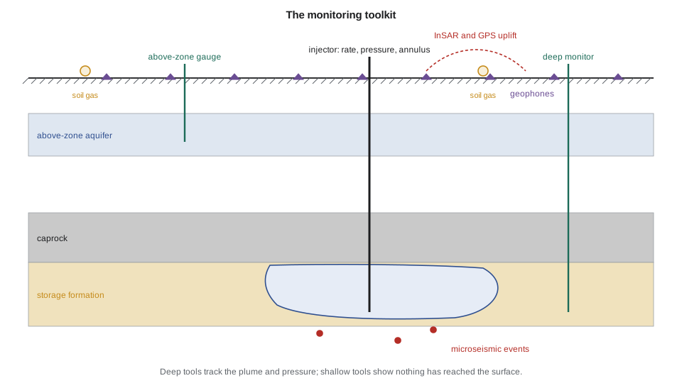
Deep monitoring: the storage formation
At the injection wells, continuous measurements of rate, pressure and temperature at surface and downhole, and of annulus pressure, are the foundation of both containment and conformance. Falloff tests during planned shutdowns measure injectivity and skin. Dedicated monitoring wells in the storage formation, some distance from the injectors, record pressure and, with pulsed neutron logs run through casing, the CO₂ saturation as the plume arrives. Fiber-optic cables cemented behind casing give distributed temperature and acoustic sensing along the whole well, which can detect flow behind casing and be used as a dense seismic receiver array.
Time-lapse, or 4D, seismic is the main tool for mapping the plume. CO₂ replacing brine lowers the rock's acoustic impedance markedly even at low saturation, so repeat surveys show where the plume is. At Sleipner, surveys since 1999 have mapped the plume in detail. The response saturates at low CO₂ saturations, so seismic maps the plume's extent better than the amount of CO₂ in each part of it. Vertical seismic profiles from monitoring wells give higher resolution near the wells at lower cost. Repeat surveys are expensive, so their frequency is set by how fast the plume changes: often every two to five years.
Above the seal
The most sensitive early warning of a leak through the seal or along a well is often pressure in the first permeable zone above it, the above-zone monitoring interval. If CO₂ or brine escapes from the storage zone, the pressure in that zone rises long before CO₂ itself reaches any monitoring well. Permanent quartz gauges resolve pressure changes of well under a kilopascal after correcting for earth tides and barometric effects. The code below estimates how large a leak would have to be for those gauges to see it.
# Above-zone pressure monitoring: could a monitoring well detect brine leaking up a degraded legacy wellbore?
# Then a simple measurement, monitoring and verification (MMV) budget for the hub.
import math
SI = False     # True: Canadian hub, metric; False: US hub, US units

def E1(u):
    s, term, n = -0.5772156649 - math.log(u), 1.0, 1
    while True:
        term *= -u / n; add = -term / n; s += add; n += 1
        if abs(add) < 1e-14: return s

# leak path: degraded cement annulus between the storage zone and the first permeable zone above the seal
area = 0.01                      # m2 of degraded annulus
L = 300.0 if SI else 250.0       # m of seal and overburden crossed
dp_store = 4.0e6 if SI else 3.1e6   # Pa of buildup at the legacy well, from the injection model
mu = 7.5e-4 if SI else 4.5e-4
def leak(k_md): return k_md * 9.869e-16 * area * dp_store / (mu * L)     # m3/s of brine
for k_md, lab in ((0.001, "sound cement"), (1.0, "cracked cement"), (1000.0, "open microannulus"), (1e5, "failed plug, open hole")):
    print(f"{lab:23s} {k_md:>8,g} mD: leak {leak(k_md) * 86400:9.3g} m3/day ({leak(k_md) * 86400 * 6.29:7.3g} bbl/day)")
q = leak(1e5)
print("Above-zone response for the failed-plug case (a microannulus gives 1/100 of these values):")
# above-zone aquifer that receives the leak
kA, hA, phiA, ctA = 50 * 9.869e-16, 20.0, 0.20, 1.0e-9
gauge = 0.7e3                    # Pa, practical resolution of a permanent quartz gauge with tidal and barometric correction
print(" distance to monitor   1 month    6 months   2 years   (above-zone pressure rise)")
for r in (100, 300, 600, 1000):
    row = []
    for days in (30, 180, 730):
        t = days * 86400
        dp = q * mu / (4 * math.pi * kA * hA) * E1(r * r * phiA * mu * ctA / (4 * kA * t))
        row.append(dp)
    lab = f"{r:,d} m" if SI else f"{r * 3.281:,.0f} ft"
    fmt = (lambda p: f"{p / 1e3:6.1f} kPa") if SI else (lambda p: f"{p / 6894.8:6.2f} psi")
    det = "  detectable" if row[-1] > 3 * gauge else ""
    print(f"{lab:>18s}   " + "   ".join(fmt(x) for x in row) + det)

# MMV budget: baseline, operations and post-closure items, local currency (illustrative)
items = [("baseline 3D seismic over the plume area", 6.0, "once"), ("repeat 3D seismic, every 3 years", 5.0, 3),
         ("two deep and four above-zone monitoring wells", 28.0, "once"), ("well gauges, sampling and logging", 1.2, 1),
         ("InSAR and GPS surface deformation", 0.3, 1), ("soil gas and groundwater sampling", 0.4, 1),
         ("microseismic array operation", 0.5, 1), ("data management and reporting", 0.6, 1)]
cur = "million Canadian dollars" if SI else "million US dollars"
total = 0.0
for name, cost, freq in items:
    life = cost if freq == "once" else cost * 25 / freq
    total += life
    print(f"  {name:48s} {cost:5.1f} {'once' if freq == 'once' else 'per ' + str(freq) + ' yr':>9s}  25-yr {life:6.1f}")
print(f"Total over 25 years: {total:.0f} {cur}, about {total / 75:.2f} per metric ton stored")sound cement 0.001 mD: leak 2.35e-08 m3/day (1.48e-07 bbl/day)
cracked cement 1 mD: leak 2.35e-05 m3/day (0.000148 bbl/day)
open microannulus 1,000 mD: leak 0.0235 m3/day ( 0.148 bbl/day)
failed plug, open hole 100,000 mD: leak 2.35 m3/day ( 14.8 bbl/day)
Above-zone response for the failed-plug case (a microannulus gives 1/100 of these values):
distance to monitor 1 month 6 months 2 years (above-zone pressure rise)
328 ft 0.83 psi 1.08 psi 1.28 psi detectable
984 ft 0.51 psi 0.77 psi 0.97 psi detectable
1,969 ft 0.32 psi 0.57 psi 0.77 psi detectable
3,281 ft 0.19 psi 0.43 psi 0.62 psi detectable
baseline 3D seismic over the plume area 6.0 once 25-yr 6.0
repeat 3D seismic, every 3 years 5.0 per 3 yr 25-yr 41.7
two deep and four above-zone monitoring wells 28.0 once 25-yr 28.0
well gauges, sampling and logging 1.2 per 1 yr 25-yr 30.0
InSAR and GPS surface deformation 0.3 per 1 yr 25-yr 7.5
soil gas and groundwater sampling 0.4 per 1 yr 25-yr 10.0
microseismic array operation 0.5 per 1 yr 25-yr 12.5
data management and reporting 0.6 per 1 yr 25-yr 15.0
Total over 25 years: 151 million US dollars, about 2.01 per metric ton storedThe result is sobering and useful. A cracked cement sheath of about 1 mD effective permeability leaks so little brine that no pressure gauge could see it, and it would also matter little. An open microannulus leaks about a hundredth of a cubic meter a day, still below detection at any distance. A failed plug or open borehole, the kind of failure that would matter, leaks 2.3 m³ a day and raises the above-zone pressure by several kilopascals within months at distances up to a kilometer, well above the gauge resolution. Above-zone pressure monitoring therefore catches the significant failures quickly. Small leaks need other tools, chiefly geochemical sampling of the above-zone water for dissolved CO₂ and brine tracers, logging of the wells themselves, and soil gas surveys at the wellheads. Amara's design placed above-zone gauges near the legacy wells with the weakest records.
Worked problem
Is a gauge response a leak?
An above-zone gauge 2,000 ft from a legacy well shows a rise of 0.62 psi over six months, after tidal and barometric correction. The code above predicts 0.57 psi at that distance and time for a leak of about 15 bbl/day from the storage zone. Gauge resolution is 0.1 psi. What should the operator do?
Show solution
- The signal is about six times the resolution, so it is real.
- It matches the size expected for a significant leak at the nearest weak well, so a leak is the leading explanation.
- Other causes must be checked: a change in nearby water production, a disposal well, or a gauge drift.
- The response plan would sample the above-zone water for CO₂ and brine tracers, log the legacy well, and if confirmed, reduce injection near it and plan remediation.
Answer: Treat it as a possible leak, confirm with independent data, and respond in proportion. The value of the gauge is that it gives months of warning while the leak is still small.
Near-surface and surface monitoring
Shallow monitoring has a different job: to show that nothing has reached groundwater or the surface, and to detect it if something does. Groundwater sampling in domestic and dedicated monitoring wells tracks pH, alkalinity, dissolved CO₂, major ions and trace metals that could be mobilized by CO₂ or brine. Soil gas surveys measure CO₂ and its ratio to oxygen and nitrogen; process-based methods, which compare the gases that would be consumed or produced by natural respiration, distinguish leakage from biology better than CO₂ concentration alone. Atmospheric methods, such as eddy covariance towers and open-path lasers, can detect larger releases over an area. Stable carbon isotopes and added tracers help attribute any anomaly. Most of these tools are run around wells and along faults, where leakage is most likely, rather than evenly over the whole area.
Satellite interferometric radar (InSAR) measures ground surface movement to a few millimeters over large areas, showing the pressure footprint as a gentle uplift; at In Salah it revealed the fracture zone discussed in Lesson 9. GPS stations and tiltmeters provide continuous point measurements. A microseismic network of surface and borehole geophones records small earthquakes; their locations and magnitudes show whether injection is stressing faults or the seal.
| Tool | What it detects | Purpose | Typical frequency |
|---|---|---|---|
| Injection rate, pressure, temperature | injectivity, well integrity | conformance, containment | continuous |
| Annulus pressure | tubing or packer leaks | containment | continuous |
| Pulsed neutron logs | CO₂ saturation near wells | conformance | yearly |
| 4D seismic or VSP | plume extent | conformance | every 2–5 years |
| Above-zone pressure | leakage through seal or wells | containment | continuous |
| Above-zone fluid sampling | CO₂ and brine tracers | containment | yearly |
| Groundwater and soil gas | near-surface impact | containment, assurance | quarterly to yearly |
| InSAR and GPS | pressure footprint, uplift | conformance | monthly |
| Microseismic array | fault activation, seal integrity | containment | continuous |
Accounting and verification
For credits, the metric tons must be measured and the stored quantity verified. Metering at custody transfer points and at each well measures the mass injected, with flow meters calibrated for dense CO₂ and composition analysis to count only CO₂. Losses between the meters and the formation, such as venting during maintenance and equipment leaks, are subtracted. Under the US 45Q credit, storage in saline formations must be documented through the EPA Greenhouse Gas Reporting Program's Subpart RR, which requires an approved monitoring, reporting and verification (MRV) plan describing how leakage would be detected and quantified and annual reports of the mass injected and stored; storage associated with enhanced oil recovery can use Subpart RR or the ISO 27916 standard. Credits can be recaptured if CO₂ is later found to have leaked during a recapture period.
Cost and adaptation
The budget from the code, about 150 million US dollars over 25 years or roughly 2 dollars per metric ton, is typical: monitoring is a small part of the cost per metric ton but a large and visible part of a hub's operating budget. Most of it goes to seismic and monitoring wells. A good program is adaptive: it monitors more intensively early, when uncertainty and risk are highest, and reduces frequency as conformance is demonstrated, with regulatory approval. The Illinois Basin–Decatur project and other Class VI projects similarly revised their monitoring as data accumulated. After injection ends, monitoring continues until the regulator accepts that the plume is stable, the condition for closure discussed in Lesson 11.
Common mistakes
MistakeChoosing tools before identifying risks.
InsteadStart from the risk assessment: list pathways, then choose tools with the sensitivity and timing to detect each.
MistakeSkipping or shortening the baseline.
InsteadCollect at least a year of baseline data, especially for soil gas and groundwater, which vary naturally.
MistakeExpecting 4D seismic to quantify CO₂ mass in the plume.
InsteadSeismic maps extent well but saturates at low CO₂ saturation; use it with logs, pressure and models.
MistakeRelying on surface monitoring to detect leaks early.
InsteadAbove-zone pressure and well monitoring give earlier warning; surface tools confirm and assure.
Summary and key terms
- MMV serves containment, conformance, accounting and public assurance, and is designed from the risk assessment.
- A baseline of at least a year is needed for every measured quantity.
- Deep monitoring uses well data, monitoring wells, saturation logs, fiber optics and 4D seismic.
- Above-zone pressure is the most sensitive early warning of significant leakage through wells or the seal.
- Shallow monitoring of groundwater, soil gas and the atmosphere shows that nothing has reached the surface.
- Accounting for credits requires metering, loss estimation and approved quantification plans and verification.
- MMV
- Measurement, monitoring and verification of stored CO₂.
- Conformance
- Agreement between observed and predicted behavior of the plume and pressure.
- Above-zone monitoring interval
- The first permeable zone above the seal, monitored for pressure and fluid changes.
- 4D seismic
- Repeated 3D seismic surveys used to track changes such as plume growth.
- InSAR
- Satellite radar interferometry that measures small changes in ground elevation.
- Subpart RR
- The US EPA reporting rule for geologic sequestration used to document storage for credits.
Practice problems
Work each problem on paper first, then reveal the answer to check.
Why is at least a year of soil gas baseline needed?
Show answer
Soil CO₂ varies seasonally with temperature, moisture and biological activity.
Which tool gives the earliest warning of a large leak along a legacy well?
Show answer
Above-zone pressure monitoring near the well.
Why does 4D seismic map plume extent better than CO₂ mass?
Show answer
The seismic response saturates at low CO₂ saturation, so more CO₂ in a place changes it little.
Name two things that must be subtracted from metered CO₂ to report stored metric tons.
Show answer
Venting during maintenance and equipment leaks between the meter and the formation.
Lesson quiz · 5 questions
Score 60% or more to complete this lesson.
Create a free account to save your progress, take quizzes and earn a certificate.