Gas lift

For the 4-22H, gas lift is the plan for the high-rate years, from about month 5 until about month 30. The pad already has a gas lift compressor serving the sister well, and the gathering company will take the extra gas. 'Gas lift is simple downhole and forgiving of gas and sand,' Marisol says, 'but it is easy to waste gas. Design the valves properly and find the injection rate that actually pays.'

This lesson covers how gas lift works, continuous and intermittent gas lift, the downhole equipment, the unloading process and valve design, the depth of the operating valve, the gas-lift performance curve and its economic optimum, and how gas is allocated among wells.

How gas lift works

Gas lift injects high-pressure gas into the production tubing at depth. The gas mixes with the produced fluid, lowers the density of the column above the injection point and expands as it rises, helping to carry the liquid. Lesson 4 showed that the weight of the fluid column is the largest part of the pressure needed at the bottom of a well, so lightening it lowers the required bottomhole pressure and lets the reservoir deliver more fluid.

In continuous gas lift, gas is injected steadily, and the well flows like a naturally flowing well with a higher gas-liquid ratio. It suits wells with good productivity and enough reservoir pressure to support a substantial fluid column, typically wells producing more than about 30 m³/d or a few hundred barrels a day. In intermittent gas lift, gas is injected periodically in large volumes under a slug of liquid that has accumulated in the tubing, pushing it to surface. It suits wells with low productivity or low reservoir pressure, but it is less efficient and harder on equipment. Plunger-assisted gas lift combines a plunger with intermittent injection to reduce liquid fallback.

Gas lift has many advantages. Downhole it has no moving parts other than the valves, so it tolerates sand and solids. It handles high gas-liquid ratios, because formation gas helps rather than hinders. It works in deviated and horizontal wells. Valves can be replaced by wireline without pulling the tubing. And its rate can be adjusted easily at surface by changing the injection rate. Its disadvantages are the need for a reliable supply of high-pressure gas and compression, its limited ability to draw down the bottomhole pressure in low-pressure wells, and its low energy efficiency compared with pumps.

Equipment

Gas is supplied from a compressor through an injection line to the wellhead, where a choke or flow controller sets the rate, and down the casing-tubing annulus. A packer seals the annulus below the deepest valve. Along the tubing, gas-lift mandrels hold the valves, either in side pockets that allow wireline retrieval or on the outside of the tubing.

The most common valves are injection-pressure-operated (IPO) valves, also called casing-pressure-operated valves. Each has a bellows charged with nitrogen at a set pressure. When the injection gas pressure in the annulus acts on the bellows with enough force to overcome the charge, the valve opens and gas passes into the tubing; when the annulus pressure falls, it closes. Production-pressure-operated valves respond mainly to tubing pressure instead. The deepest valve, where gas is injected during normal operation, is often an orifice valve, which is always open and simply meters gas, preceded by a check valve to stop backflow.

Unloading the well

When a gas-lifted well is started, or restarted after a shutdown, its annulus and tubing are full of liquid, often kill fluid or water. The available gas pressure cannot push all that liquid out through the deepest valve at once. Instead, the valves are spaced so that the well is unloaded from the top down. Gas injected into the annulus pushes liquid down the annulus and up through the open valves into the tubing. When the liquid level in the annulus reaches the top valve, gas enters the tubing there and lightens the column above it, which lowers the tubing pressure at the next valve down. The annulus liquid then drops to the second valve, gas enters there, and the top valve closes because the annulus pressure has been lowered slightly by design. The process continues until gas reaches the operating valve.

Valve spacing is designed graphically or with software. The engineer draws the injection gas pressure line, the static and flowing gradients of the well fluid, and the unloading gradient, and places each valve where the tubing pressure, lightened by gas above the previous valve, allows the annulus liquid to fall far enough. Each valve's opening pressure is set slightly lower than the one above it, typically 10 to 25 psi or about 70 to 170 kPa lower, so that upper valves close in turn as the injection point moves down.

The operating injection depth

The deepest point at which gas can enter the tubing in continuous operation is where the injection gas pressure, less a margin for the pressure drop across the valve, equals the flowing tubing pressure. Below that point, the tubing pressure is higher than the gas pressure and gas cannot enter. The deeper the injection point, the more of the column is lightened and the lower the bottomhole pressure, so higher injection pressure is valuable.

The gas pressure at depth is higher than at surface because of the weight of the gas column, which increases roughly exponentially with depth for a given gas gravity and temperature. The tubing pressure below the injection point follows the gradient of the unaerated well fluid upward from the flowing bottomhole pressure.

# Gas lift: depth of the operating injection point, and the economic optimum injection rate
import math
SI = False  
if SI:   # 04-22 Cardium gas-lift option at month 6; internal field units, shown in SI
    D_ft, pso, sg_g, T_R, pwf_target, grad_below, dpv = 4757.0, 5500 * 0.145038, 0.75, 560.0, 6000 * 0.145038, 0.36, 100.0
    qmax, a, b, oil_frac, netback, gas_cost = 300.0, 0.012, 0.035, 0.75, 330 / 6.2898, 3.0
    sp = lambda p: f"{p / 0.145038:,.0f} kPa"; sd = lambda f: f"{f * 0.3048:,.0f} m"
    sq = lambda b: f"{b / 6.2898:,.1f} m3/d"; sg_ = lambda m: f"{m * 28.317:,.0f} m3/d"
    sm = lambda r: f"{r * 5.615:.1f} m3 oil per 1,000 m3 gas"
else:    # 4-22H Bakken gas lift at month 6
    D_ft, pso, sg_g, T_R, pwf_target, grad_below, dpv = 10100.0, 1400.0, 0.90, 620.0, 2200.0, 0.37, 100.0
    qmax, a, b, oil_frac, netback, gas_cost = 1500.0, 0.0028, 0.10, 0.58, 40.0, 3.0
    sp = lambda p: f"{p:,.0f} psi"; sd = lambda f: f"{f:,.0f} ft"; sq = lambda b: f"{b:,.0f} bbl/d"; sg_ = lambda m: f"{m:,.0f} Mscf/d"
    sm = lambda r: f"{r:.2f} bbl oil per Mscf"
# injection-gas pressure at depth (static gas column, average z about 0.85)
def p_gas(z): return (pso + 14.7) * math.exp(0.01875 * sg_g * z / (0.85 * T_R)) - 14.7
# tubing pressure at depth below the injection point: pwf minus the liquid gradient up from the bottom
def p_tub(z): return pwf_target - grad_below * (D_ft - z)
z = 0.0
while z + 10 <= D_ft and p_gas(z + 10) - dpv >= p_tub(z + 10): z += 10   # deepest point where gas can still enter
print(f"surface injection pressure {sp(pso)}; injection gas is at {sp(p_gas(z))} at {sd(z)}")
if z + 10 > D_ft:
    print(f"the gas can enter at the bottom of the tubing ({sd(D_ft)}) for a flowing pressure of {sp(pwf_target)}")
else:
    print(f"deepest operating injection point about {sd(z)}: below it the tubing pressure exceeds the gas pressure less a {sp(dpv)} valve drop")
# performance curve: gross liquid rate versus injection rate (a fitted shape), and the economic optimum
qg_list = [0, 100, 200, 400, 600, 800, 1000, 1400] if not SI else [0, 30, 60, 100, 150, 200, 300, 400]
f = lambda g: qmax * (1 - math.exp(-a * g)) - b * g
print("   injection gas      gross liquid      extra oil per extra gas")
prev = None
for g in qg_list:
    q = f(g); txt = "" if prev is None else sm((q - prev[1]) * oil_frac / (g - prev[0]))
    print(f"   {sg_(g):>14s}   {sq(q):>16s}   {txt}"); prev = (g, q)
# optimum: d(oil value)/dg = gas cost  ->  qmax*a*exp(-a g) - b = gas_cost / (oil_frac * netback)
target = gas_cost / (oil_frac * netback) + b
g_opt = math.log(qmax * a / target) / a
g_max = math.log(qmax * a / b) / a
print(f"maximum liquid at about {sg_(g_max)}; economic optimum at about {sg_(g_opt)} giving {sq(f(g_opt))} gross")

surface injection pressure 1,400 psi; injection gas is at 1,868 psi at 8,930 ft
deepest operating injection point about 8,930 ft: below it the tubing pressure exceeds the gas pressure less a 100 psi valve drop
   injection gas      gross liquid      extra oil per extra gas
         0 Mscf/d            0 bbl/d   
       100 Mscf/d          356 bbl/d   2.07 bbl oil per Mscf
       200 Mscf/d          623 bbl/d   1.55 bbl oil per Mscf
       400 Mscf/d          971 bbl/d   1.01 bbl oil per Mscf
       600 Mscf/d        1,160 bbl/d   0.55 bbl oil per Mscf
       800 Mscf/d        1,260 bbl/d   0.29 bbl oil per Mscf
     1,000 Mscf/d        1,309 bbl/d   0.14 bbl oil per Mscf
     1,400 Mscf/d        1,330 bbl/d   0.03 bbl oil per Mscf
maximum liquid at about 1,335 Mscf/d; economic optimum at about 1,038 Mscf/d giving 1,314 bbl/d gross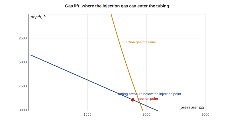

For the 4-22H, with a target bottomhole pressure of 2,200 psi and a surface injection pressure of 1,400 psi from the pad compressor, gas can enter the tubing down to about 8,930 ft, below which the tubing pressure exceeds the gas pressure. The packer and lowest mandrel will be set near 9,000 ft, at the top of the curve, so injection takes place as deep as the gas pressure allows.

The gas-lift performance curve

Injecting more gas lightens the column further, so the rate rises, but each additional unit of gas brings less extra liquid than the one before. Eventually the extra gas adds more friction than it removes in weight, and the rate begins to fall. Plotting liquid rate against injection rate gives the gas-lift performance curve, which rises steeply, flattens, peaks and then declines.

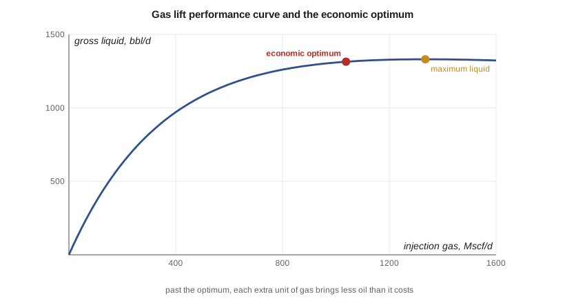
The technical maximum is the injection rate at the top of the curve. The economic optimum is lower: it is the rate at which the value of the extra oil from one more unit of gas equals the cost of that gas, including compression, fuel and the value the gas could earn if sold. In mathematical terms, the slope of the curve times the oil fraction times the oil netback equals the gas cost.

For the 4-22H, the curve shows that the first 100 Mscf/d of gas lifts about 356 bbl/d, but by 800 Mscf/d each additional Mscf brings only about 0.3 bbl of oil. The technical maximum is near 1,335 Mscf/d; the economic optimum, with gas valued at about 3 dollars per Mscf and an oil netback of 40 dollars per barrel, is about 1,040 Mscf/d, giving about 1,314 bbl/d of gross liquid. Because the curve is so flat near the top, the last 300 Mscf/d of gas adds only about 20 bbl/d of liquid.

Allocating gas among wells

In a field with several gas-lifted wells sharing a compressor, the available gas is limited, and the question becomes how to divide it. The optimum allocation gives each well gas until the marginal oil per unit of gas is the same in every well. A well with a steep curve should get more gas, and a well near the flat top of its curve should get less. Many fields use automated optimizers that read each well's test data and adjust injection rates daily. Simply giving every well the same injection rate, or giving each well its technical maximum until the gas runs out, can waste a large share of the gas.

Gas lift also needs regular surveillance. Common problems include multipointing, where gas enters through more than one valve, a sign that an upper valve is not closing; heading, where injection and production surge in cycles; and valves that are cut out or leaking. Flowing pressure surveys, temperature logs and acoustic surveys identify which valve is injecting, and wireline crews replace faulty valves.