Inflow from horizontal and fractured wells

The Tamarack 4-22H horizontal well is nothing like the vertical well of lesson 2. Its lateral runs about 10,000 ft through the Bakken, where matrix permeability is measured in microdarcies, and it was fractured in 50 stages. 'Vogel was built for vertical wells in a tank,' Marisol says. 'Your horizontal well drains a long, thin slab of rock through hundreds of fractures, and its productivity is still changing. You need a different way of thinking about its inflow.'

This lesson explains how horizontal wells and hydraulic fractures change the geometry of flow, how their productivity is estimated with Joshi's equation and the effective wellbore radius of a fracture, and why a multistage fractured horizontal well in tight rock has a transient IPR that shrinks for months or years. It ends with how production engineers use the well's own data to build an IPR they can trust.

Why geometry matters

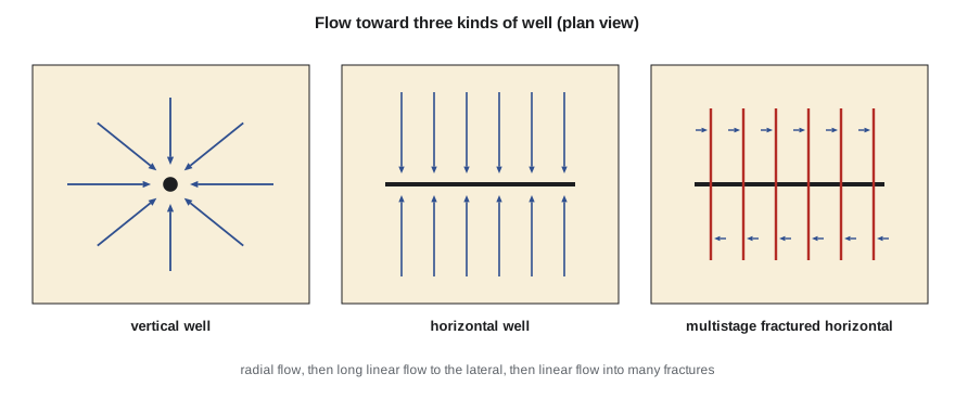
In a vertical well, flow converges radially. The pressure drop is concentrated close to the well, where the area open to flow is smallest, which is why skin has such a large effect and why productivity grows only with the logarithm of the drainage radius. A horizontal well changes this picture. Flow near the lateral is roughly linear rather than radial, the area open to flow is the length of the lateral times the formation thickness, and the pressure drop near the well is much smaller for the same rate. Hydraulic fractures go further, creating planes of very high conductivity that extend tens or hundreds of meters into the rock and turn almost all of the flow into linear flow toward the fracture faces.

These geometries change both the size of the IPR and how it evolves with time. In low-permeability rock, the pressure disturbance from a well spreads slowly. A vertical well in such rock may take years to reach pseudosteady state, and a fractured horizontal well may spend most of its life in transient linear flow, with its productivity falling as the square root of time.

Horizontal wells: Joshi's equation

Several engineers derived steady-state and pseudosteady-state productivity equations for horizontal wells in the 1980s and 1990s. The most widely used is Joshi's, which treats the drainage volume as an ellipse around the lateral and adds a term for the vertical convergence of flow into the wellbore.

Here L is the lateral length, a is the half major axis of the drainage ellipse, which depends on L and the drainage radius, and β is the square root of the ratio of horizontal to vertical permeability. The first logarithm describes flow toward the lateral from the far reservoir; it is small because the lateral is long. The second term describes the convergence of flow from the formation thickness into the small wellbore, and it grows when vertical permeability is low. Laminations and shale streaks, common in many tight formations, cut vertical permeability and hurt unfractured horizontal wells more than any other factor.

Joshi's equation and its relatives assume an undamaged lateral with full contact along its length, steady or pseudosteady flow and a homogeneous reservoir. Real laterals are often damaged by days of exposure to drilling mud, may be partly blocked by cuttings beds or water, and drain unevenly because of friction along the lateral. Their measured productivity is often well below the ideal value.

Hydraulically fractured vertical wells

A single vertical fracture acts like a much larger wellbore. Prats showed that a fracture of infinite conductivity with half-length xf behaves, in pseudosteady state, like a well with an effective wellbore radius of xf/2. Substituting that radius into the radial equation gives the productivity of a fractured vertical well. For a fracture of finite conductivity, the effective radius is smaller and depends on the dimensionless fracture conductivity CfD, as PET-330 showed. In skin terms, a good fracture gives a strongly negative skin, typically between about −3 and −6.

Comparing the geometries

# Horizontal and fractured-well inflow: Joshi for an unfractured lateral, Prats for a fractured vertical well,
# and a transient IPR for the multistage-fractured horizontal well calibrated to its own early test
import math
SI = False  
# rock and fluid data in field units for the equations (ft, md, cp)
if SI:   # Cardium tight flank, 04-22
    k, h, mu, B, rw, L, reh, kvkh = 0.5, 21.3, 0.8, 1.29, 0.25, 6824.0, 1640.0, 0.1
    J30, pr_t, pb, tel = 52.0 / 4350.0, [(1, 14600), (6, 13600), (12, 12900), (24, 11800)], 12800.0, 45
    pu, ru, conv = "kPa", "m3/d", 6.2898 * 6.89476   # 1 m3/d per kPa = 43.4 STB/d per psi
else:    # Bakken, 4-22H
    k, h, mu, B, rw, L, reh, kvkh = 0.01, 45.0, 0.4, 1.50, 0.25, 10000.0, 1320.0, 0.1
    J30, pr_t, pb, tel = 1050.0 / 1000.0, [(1, 5300), (6, 4700), (12, 4200), (24, 3600)], 2600.0, 540
    pu, ru, conv = "psi", "STB/d", 1.0
re_v = reh
Jv = k * h / (141.2 * B * mu * (math.log(re_v / rw) - 0.75))            # vertical well, no skin
a = (L / 2) * math.sqrt(0.5 + math.sqrt(0.25 + (2 * reh / L) ** 4))
beta = math.sqrt(1 / kvkh)
Jh = k * h / (141.2 * B * mu * (math.log((a + math.sqrt(a * a - (L / 2) ** 2)) / (L / 2)) + beta * h / L * math.log(beta * h / (2 * rw))))
xf = 200.0
Jf = k * h / (141.2 * B * mu * (math.log(re_v / (xf / 2)) - 0.75))      # infinite-conductivity fracture, rw' = xf/2
print(f"unfractured vertical well J = {Jv / conv:.4f}  (in {ru} per {pu})")
print(f"unfractured horizontal well J (Joshi, L = {L:,.0f} ft) = {Jh / conv:.4f}, {Jh / Jv:.1f} times the vertical well")
print(f"vertical well with one {xf:.0f} ft fracture (Prats rw' = xf/2) J = {Jf / conv:.4f}, {Jf / Jv:.1f} times")
print(f"multistage fractured horizontal well, measured at day 30: J = {J30:.4f}, {J30 * conv / Jv:.0f} times the vertical well")
print("transient IPR of the multistage well (J falls as 1/sqrt(t) until fractures interfere, then levels off):")
for m, pr in pr_t:
    t = 30.4 * m
    J = J30 * math.sqrt(30.4 / min(t, tel))
    qb = J * max(pr - pb, 0); aof = qb + J * min(pr, pb) / 1.8
    print(f"   month {m:2d}: pr {pr:6,} {pu}  J {J:.4f}  AOF {aof:7.1f} {ru}")

unfractured vertical well J = 0.0007  (in STB/d per psi)
unfractured horizontal well J (Joshi, L = 10,000 ft) = 0.0354, 52.2 times the vertical well
vertical well with one 200 ft fracture (Prats rw' = xf/2) J = 0.0029, 4.3 times
multistage fractured horizontal well, measured at day 30: J = 1.0500, 1546 times the vertical well
transient IPR of the multistage well (J falls as 1/sqrt(t) until fractures interfere, then levels off):
   month  1: pr  5,300 psi  J 1.0500  AOF  4351.7 STB/d
   month  6: pr  4,700 psi  J 0.4287  AOF  1519.4 STB/d
   month 12: pr  4,200 psi  J 0.3031  AOF   922.8 STB/d
   month 24: pr  3,600 psi  J 0.2491  AOF   609.0 STB/d

The comparison for the Bakken is instructive. An unfractured vertical well in this rock would have a J of only about 0.0007 STB/d per psi, far too low to be economic. A single 200 ft fracture multiplies it by about 4. An ideal unfractured 10,000 ft lateral would multiply it by about 50, and the 4-22H as measured at day 30 has more than a thousand times the vertical well's productivity. In rock this tight, the fractures are everything: the matrix delivers fluid only over very short distances, and the hundreds of fracture faces provide the area that makes the well work.

Transient inflow: an IPR that shrinks

In tight rock, the IPR of a fractured horizontal well is not a fixed curve. Early in its life the well draws on the rock right next to each fracture face. The pressure disturbance moves away from the faces with time, the region feeding each fracture grows more slowly than the time, and the productivity falls roughly in proportion to one over the square root of time. This period of transient linear flow ends when the disturbances from neighboring fractures meet, after which the region between fractures depletes as a whole and the well enters a boundary-dominated period in which productivity is nearly constant but reservoir pressure falls steadily.

The time to the end of linear flow depends on the permeability and the spacing between fractures. In rock of a few tenths of a millidarcy with fractures 20 m apart, interference comes within weeks; in rock of a few microdarcies, it can take years. Many unconventional wells are still in linear flow when they are first put on artificial lift, so the lift design must allow for inflow that keeps falling.

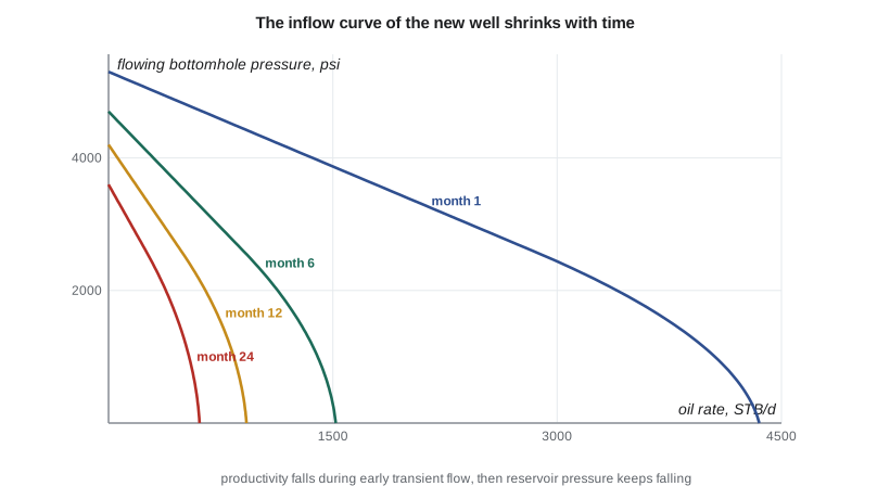
For the 4-22H, the program calibrates J to the day-30 test and assumes that linear flow lasts about 18 months, a typical figure for Bakken wells at this fracture spacing. J falls from about 1.05 STB/d per psi at month 1 to about 0.43 at month 6, 0.30 at month 12 and 0.25 at month 24. Together with the falling reservoir pressure, the AOF shrinks from more than 4,000 STB/d to about 1,500, then 920, then 610 STB/d. These AOFs are well above what the well actually makes, because the tubing cannot draw the bottomhole pressure down to zero. Lesson 6 combines these curves with the tubing to find the actual rates.

Building an IPR from production data

Because analytical equations for fractured horizontal wells depend on many uncertain inputs, such as effective fracture half-length, the number of fractures that actually contribute and the permeability between them, production engineers lean heavily on each well's own data. The key measurement is the flowing bottomhole pressure, either from a permanent downhole gauge or calculated from wellhead pressure and a tubing model. With rate and pressure recorded daily, the engineer can plot a rate-normalized pressure, the drawdown divided by the rate, against the square root of time. A straight line confirms linear flow, its slope gives the product of fracture area and the square root of permeability, and a bend upward marks the end of linear flow.

These analyzes, known as rate transient analysis, are covered in detail in PET-360. For the production engineer, the practical result is a set of J values at different times and a model of how J will evolve, which is all that a lift design needs.

Ethan notes that the 4-22H has a pressure gauge at the heel, installed by Tom's completions team in PET-330. That single decision makes his work much easier: he can watch J fall in real time and see whether the 18-month estimate for linear flow holds.

Flow along the lateral

One more effect matters in long laterals: the pressure drop along the lateral itself. Fluid entering near the toe must travel thousands of meters or feet to reach the heel. At high rates, friction along the lateral reduces the drawdown at the toe, so the toe contributes less than the heel. In toe-up laterals, liquid can collect in low spots and gas can collect in high spots, causing slugging; in toe-down laterals, water can settle near the toe. Production logs and tracers from PET-330 show that in the Tamarack Lake field, heel stages typically contribute more than toe stages. Lift equipment is usually set in the vertical section or the curve above the lateral, so the lateral must carry fluid to the pump intake by itself.