Nodal analysis

Ethan now has both halves of the production system for the Tamarack 4-22H horizontal well: a transient inflow curve from lesson 3 and an outflow curve from lesson 4. Marisol asks three questions. 'At what rate should the well be flowing today, and does that match the test? How long will it keep flowing on its own? And what could we change to make it flow longer or faster?' The method that answers all three is nodal analysis, sometimes called systems analysis.

This lesson explains the idea of a solution node, how the operating point is found where inflow and outflow meet, how stability is judged, and how sensitivity studies on tubing size, wellhead pressure, skin and water cut guide decisions. It then applies the method to the new well over its first two years to find when artificial lift will be needed.

The idea of a node

Nodal analysis treats the production system as a chain of components connected at points called nodes: the average reservoir pressure, the sandface, the bottom of the tubing, the wellhead, the downstream side of the choke and the separator. At any node, the pressure arriving from upstream must equal the pressure required by the downstream part of the system, and the rate through every component must be the same. The engineer picks one node as the solution node, calculates the pressure there from the upstream end for a range of rates, calculates it again from the downstream end for the same rates, and looks for the rate at which the two agree.

The most common solution node is the bottom of the tubing, near the sandface. The upstream calculation is the IPR: for each rate, the flowing bottomhole pressure the reservoir can provide. The downstream calculation is the outflow curve: for each rate, the bottomhole pressure needed to push the fluid up the tubing and through the surface system to the separator. Plotted together, the two curves cross at the operating point, which gives the predicted rate and bottomhole pressure.

Other nodes are used for other questions. Putting the node at the wellhead separates the subsurface from the surface, which is useful for choke and flowline studies. Putting it at the sandface separates the completion from the reservoir, which helps evaluate perforating or stimulation. The answer, the operating rate, is the same whichever node is chosen, because the same equations are being solved; the choice only changes which effects are easiest to see.

Stability

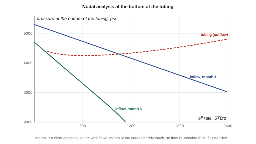
The IPR falls with rate, and the outflow curve falls at low rates and rises at high rates. The two curves can therefore cross twice. The crossing on the right, where the outflow curve is rising, is the stable operating point: if the rate rises slightly, the outflow pressure needed exceeds the inflow pressure available, so the rate falls back, and the reverse happens if the rate falls. The crossing on the left, on the falling side of the outflow curve, is unstable: a small drop in rate makes the column heavier, which reduces the rate further until the well dies or begins to head. When the curves do not cross at all, the well cannot flow, and it needs lift.

Engineers watch the distance between the operating point and the minimum of the outflow curve. A well operating close to the minimum is near the edge of stability, and small disturbances, such as a slug of water or a rise in line pressure, can kill it. Wells in that condition often benefit from smaller tubing, lower wellhead pressure or early installation of lift.

Nodal analysis for the new well

The program combines the transient IPR of lesson 3 with the outflow model of lesson 4. At each time it inverts the IPR to find the pressure available at each rate, compares it with the pressure the tubing needs, and finds the stable crossing if there is one. It repeats the calculation for a smaller or larger tubing and for a lower wellhead pressure.

# Nodal analysis at the bottom of the tubing: where the inflow curve (IPR) meets the outflow curve (tubing),
# for the new horizontal well over its first two years, with tubing and wellhead pressure sensitivities
import math
SI = False  
g = 9.81
if SI:   # 04-22 Cardium; internal units SI (kPa, m3/d)
    depth, T1, T2, ro, rw_, sg = 1500.0, 20.0, 55.0, 835.0, 1050.0, 0.75
    gor, rsb, pb = 108.0, 100.0, 12800.0
    life = [(1, 14600, 0.0120, 0.21), (6, 13600, 0.0098, 0.25), (12, 12900, 0.0098, 0.30), (24, 11800, 0.0098, 0.38)]
    pwh0, D0, Dalt = 1450.0, 0.0620, 0.0507
    fmt_p = lambda p: f"{p:,.0f} kPa"; fmt_q = lambda q: f"{q:,.1f} m3/d"; ql = lambda q: q; alt_name = "60.3 mm tubing"; lowp = 700.0
else:    # 4-22H Bakken; converted to SI inside, shown in field units
    depth, T1, T2, ro, rw_, sg = 3078.0, 15.0, 110.0, 815.0, 1150.0, 0.90
    gor, rsb, pb = 857 / 5.6146, 795 / 5.6146, 2600 * 6.89476
    life = [(m, p * 6.89476, J / 43.366, wc) for m, p, J, wc in   # J converted from STB/d per psi
            [(1, 5300, 1.05, 0.35), (6, 4700, 0.4287, 0.42), (12, 4200, 0.3031, 0.48), (24, 3600, 0.2491, 0.55)]]
    pwh0, D0, Dalt = 650 * 6.89476, 0.0620, 0.0760
    fmt_p = lambda p: f"{p / 6.89476:,.0f} psi"; fmt_q = lambda q: f"{q * 6.2898:,.0f} STB/d"; alt_name = "3-1/2 in tubing"; lowp = 250 * 6.89476
def tubing(qo, wc, pwh, D, steps=150):
    qw = qo * wc / (1 - wc); p = pwh; dz = depth / steps; A = math.pi * D * D / 4
    for i in range(steps):
        z = (i + 0.5) * dz; T = T1 + (T2 - T1) * z / depth + 273.15
        rs = rsb * min(p / pb, 1.0); free = max(gor - rs, 0.0) * qo
        vsg = free * (101.325 / p) * (T / 288.7) * 0.92 / 86400 / A
        vsl = (qo * (1 + 0.0005 * rs) + qw) / 86400 / A; vm = vsl + vsg
        rl = (ro * qo + rw_ * qw) / (qo + qw); rg = p * 1000 * 28.97 * sg / (0.92 * 8314 * T)
        vd = 1.53 * (g * 0.03 * (rl - rg) / rl ** 2) ** 0.25
        ag = vsg / (1.2 * vm + vd) if vsg > 0 else 0.0
        rm = ag * rg + (1 - ag) * rl
        p += (rm * g + 0.022 * rm * vm * vm / (2 * D)) * dz / 1000
    return p
def ipr(pwf, pr, J):
    qb = J * max(pr - pb, 0)
    if pwf >= pb: return J * (pr - pwf)
    x = pwf / min(pr, pb); return qb + J * min(pr, pb) / 1.8 * (1 - 0.2 * x - 0.8 * x * x)
def solve(pr, J, wc, pwh, D):
    best = None             # keep the right-hand crossing: the stable operating point
    qmax = ipr(0, pr, J)
    lo, hi = 0.5, qmax * 0.999
    f = lambda q: tubing(q, wc, pwh, D)
    def gap(q):          # inflow pressure available at rate q minus tubing pressure needed
        a, b = 0.0, pr   # invert the IPR by bisection
        for _ in range(50):
            m = (a + b) / 2
            if ipr(m, pr, J) > q: a = m
            else: b = m
        return a - f(q)
    qs = [lo + (hi - lo) * i / 60 for i in range(61)]
    vals = [gap(q) for q in qs]
    for (q1, v1), (q2, v2) in zip(zip(qs, vals), zip(qs[1:], vals[1:])):
        if v1 < 0 <= v2 or v1 >= 0 > v2:
            best = (q1, q2)
    if best is None: return None
    a, b = best
    for _ in range(40):
        m = (a + b) / 2
        if (gap(a) < 0) == (gap(m) < 0): a = m
        else: b = m
    q = (a + b) / 2; return q, f(q)
for m, pr, J, wc in life:
    base = solve(pr, J, wc, pwh0, D0); alt = solve(pr, J, wc, pwh0, Dalt); low = solve(pr, J, wc, lowp, D0)
    s = lambda r: "no stable flow" if r is None else f"{fmt_q(r[0])} at {fmt_p(r[1])}"
    print(f"month {m:2d} (reservoir {fmt_p(pr)}, water cut {wc:.0%}):")
    print(f"   base case                  {s(base)}")
    print(f"   {alt_name:26s} {s(alt)}")
    print(f"   lower wellhead pressure    {s(low)}")

month  1 (reservoir 5,300 psi, water cut 35%):
   base case                  1,045 STB/d at 4,304 psi
   3-1/2 in tubing            1,107 STB/d at 4,246 psi
   lower wellhead pressure    1,549 STB/d at 3,825 psi
month  6 (reservoir 4,700 psi, water cut 42%):
   base case                  no stable flow
   3-1/2 in tubing            no stable flow
   lower wellhead pressure    474 STB/d at 3,595 psi
month 12 (reservoir 4,200 psi, water cut 48%):
   base case                  no stable flow
   3-1/2 in tubing            no stable flow
   lower wellhead pressure    no stable flow
month 24 (reservoir 3,600 psi, water cut 55%):
   base case                  no stable flow
   3-1/2 in tubing            no stable flow
   lower wellhead pressure    no stable flow

At month 1 the model predicts about 1,045 STB/d at a bottomhole pressure of about 4,300 psi, matching the 1,050 STB/d measured on test, so the model is well calibrated. By month 6, with the reservoir pressure down to 4,700 psi, the productivity index less than half its day-30 value and the water cut up to 42 percent, there is no stable operating point with the current tubing and wellhead pressure: the well will be heading and dying. Larger tubing does not help. Lowering the wellhead pressure to 250 psi would keep it flowing at about 474 STB/d at month 6, but by month 12 nothing flows. The conclusion is clear: the 4-22H will need artificial lift within about six months, and with rates of several hundred barrels a day still available, the lift method must handle high volumes and high gas.

Sensitivity studies

The real value of nodal analysis lies in sensitivity studies, in which one parameter is changed at a time to see its effect on the operating rate. Typical studies include the following.

Tubing size. As lesson 4 showed, smaller tubing helps at low rates and hurts at high rates. Nodal analysis shows exactly where the crossover lies for a given well and when a tubing change would pay.

Wellhead or separator pressure. Lowering the backpressure raises the rate, sometimes dramatically in low-pressure wells. The study shows whether compression or a lower separator pressure would pay.

Skin and stimulation. Changing the skin shifts the IPR. A study at the sandface node shows how much rate a stimulation would add, which is the first step in deciding whether to acidize or refracture.

Water cut and GLR. Running the analysis at higher water cuts shows when the well will stop flowing. Running it at higher GLR shows the effect of gas lift, which is the basis of the gas-lift performance curve in lesson 9.

Reservoir pressure. Running the analysis at a series of future reservoir pressures, as the program does, gives a forecast of rate and the date when lift is needed.

Each study must be read carefully. The model is only as good as its inputs, and the inputs most likely to be wrong are the IPR at future times, the multiphase correlation and the water cut forecast. Marisol asks Ethan to rerun the analysis monthly with new test data and to state each result as a range rather than a single date.

Nodal analysis with artificial lift

Artificial lift changes the outflow side of the system. A pump adds pressure at the pump depth, so the outflow curve is shifted down by the pump's pressure rise. Gas lift reduces the density of the column above the injection point, which also shifts the outflow curve down. Nodal analysis therefore extends naturally to lift design: the engineer finds the rate at which the IPR crosses the lift-assisted outflow curve and checks that the pump or gas supply can deliver the required pressure rise or gas volume at that rate. Lessons 8 to 10 use this approach.

For pumps, the solution node is often placed at the pump intake. The upstream side is the IPR less the pressure drop from the sandface to the pump; the downstream side is the pressure the pump must deliver into the tubing, less the pressure the pump adds. The intake pressure must stay high enough to avoid excessive free gas at the pump, which is one of the most important design limits in lift.