Tubing performance and multiphase flow

Lesson 1 showed that the tubing of the 4-22H consumes about 70 percent of the available pressure. 'That makes the tubing the most important piece of equipment you can change without touching the reservoir,' Marisol says. 'The completions team ran 2-7/8 in tubing because that is what we always run. Is it the right size for this well, and will it still be right in a year?' To answer, Ethan needs the other half of the production system: the tubing performance relationship, or outflow curve.

This lesson explains the pressure gradient in a producing well, why gas and liquid flowing together are so much harder to predict than a single phase, how flow patterns and slip control the result, how the main correlations and mechanistic models work, and how tubing size affects the outflow curve.

The pressure gradient in a well

The pressure in a producing well increases with depth. Engineers split the gradient into three parts: the weight of the fluid (the elevation or hydrostatic term), friction against the pipe wall, and acceleration as the fluid speeds up when gas expands. The acceleration term is small except near the surface of high-rate gas wells, so in most oil wells the gradient is the sum of the first two.

For a single-phase liquid, every term is easy to calculate: the density is known, the velocity is the rate divided by the pipe area, and the friction factor comes from the Moody chart. The pressure increases almost linearly with depth. A column of fresh water adds about 9.8 kPa per meter (0.433 psi per foot); a 38° API oil about 8.2 kPa per meter (0.36 psi per foot); a heavy brine about 11 kPa per meter (0.49 psi per foot).

Two phases: the difficulty

Almost every oil well produces gas as well as liquid. As the fluid rises and the pressure falls, more gas comes out of solution and the free gas expands. The mixture becomes lighter toward the surface, which is exactly why gas helps a well to flow. But calculating how much lighter is difficult, for two reasons.

First, the gas and liquid do not move at the same speed. Gas, being lighter, rises faster than the liquid, a difference called slip. Because the liquid moves more slowly, it occupies a larger share of the pipe than its share of the volumetric flow. That share of the pipe cross-section occupied by liquid is the liquid holdup, and it, not the no-slip liquid fraction, sets the mixture density in the elevation term. At low rates, slip is large, holdup is high and the column is heavy; at high rates, the phases are mixed more thoroughly and slip falls.

Second, the phases arrange themselves in different flow patterns depending on the rates, pipe size, inclination and fluid properties. In bubble flow, small gas bubbles are dispersed in continuous liquid. In slug flow, large bullet-shaped gas bubbles, called Taylor bubbles, alternate with liquid slugs. In churn flow, the slugs break down into chaotic, oscillating mixtures. In annular flow, the gas flows in the core of the pipe and the liquid flows as a film on the wall and as droplets in the gas. Each pattern has its own holdup and friction behavior.

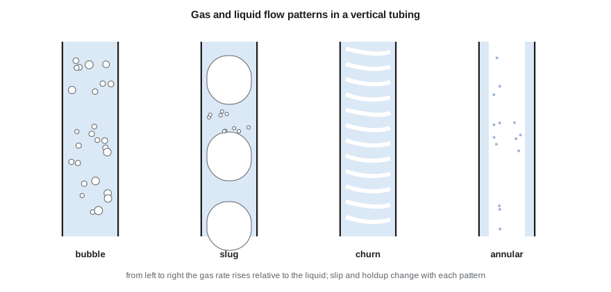
A single well can pass through several patterns. Near the bottom of the 4-22H, where pressure is above the bubble point, the flow is single-phase oil and water. Higher up, as gas comes out of solution, it is bubble flow, then slug flow, and near the surface the fast-expanding gas may push it into churn flow.

Correlations and mechanistic models

Since the 1950s, engineers have built two families of methods for the multiphase pressure gradient. Empirical correlations were fitted to laboratory or field data. Some ignore slip and flow patterns entirely (for example, Poettmann and Carpenter); others include slip but not patterns (Hagedorn and Brown, developed from tests in a 1,500 ft experimental well); and others include both (Duns and Ros, Orkiszewski, Beggs and Brill, the last developed from inclined-pipe experiments). Mechanistic models, developed from the 1980s onward, predict the flow pattern from physical criteria and then apply momentum and mass balances for that pattern; examples include those of Ansari and others and of Petalas and Aziz.

No method is best for every well. Field practice is to compare several methods against measured bottomhole pressures from gauges or surveys and choose the one that fits the field. Many companies keep a table of preferred methods for each field and type of well, and update it as gauge data accumulates. PET-380 covers these methods in detail. For production engineering, the key point is that the choice of correlation can change the predicted bottomhole pressure by 10 percent or more, which is enough to change a lift decision.

A simple model you can run

The program below uses a simplified drift-flux model. It marches down the tubing in steps, calculating at each step how much gas has come out of solution, the in-situ gas and liquid velocities, and the gas fraction from the drift-flux relation of Zuber and Findlay. That relation says the gas moves faster than the mixture by a distribution factor, about 1.2, plus a drift velocity at which bubbles rise through still liquid.

This is a teaching model. It uses a constant friction factor, a straight-line solution-gas relation and a single drift velocity, and it ignores flow-pattern transitions. It is good enough to show how tubing size, rate and gas affect the outflow curve, but field work uses a tested correlation or mechanistic model calibrated to gauges.

# Tubing performance: march down the tubing from the wellhead with a simple drift-flux model of gas and liquid,
# and compare tubing sizes and rates (a teaching model; real work uses tested correlations or mechanistic models)
import math
SI = False  
g = 9.81
if SI:   # 04-22 Cardium; depth 1,500 m to end of tubing, wellhead 1,450 kPa
    depth, pwh, T1, T2 = 1500.0, 1450.0, 20.0, 55.0
    qo, qw, gor, rsb, pb = 52.0, 14.0, 108.0, 100.0, 12800.0     # m3/d, m3/m3, kPa
    ro, rw_, sg = 835.0, 1050.0, 0.75
    sizes = [("60.3 mm (2-3/8 in)", 0.0507), ("73.0 mm (2-7/8 in)", 0.0620), ("88.9 mm (3-1/2 in)", 0.0760)]
    rates = [10, 20, 35, 52, 80, 120]
    show = lambda p: f"{p:8,.0f} kPa"; ru = "m3/d of oil"
else:    # 4-22H Bakken; depth 10,100 ft to end of tubing, wellhead 650 psi
    depth, pwh, T1, T2 = 3078.0, 650 * 6.89476, 15.0, 110.0
    qo, qw, gor, rsb, pb = 1050 / 6.2898, 560 / 6.2898, 857 / 5.6146, 795 / 5.6146, 2600 * 6.89476
    ro, rw_, sg = 815.0, 1150.0, 0.90
    sizes = [("2-3/8 in", 0.0507), ("2-7/8 in", 0.0620), ("3-1/2 in", 0.0760)]
    rates = [100, 250, 500, 1050, 1500, 2200]
    show = lambda p: f"{p / 6.89476:8,.0f} psi"; ru = "STB/d of oil"
wc = qw / (qo + qw)
def pwf(qo_m3d, D, steps=300):
    qw_m3d = qo_m3d * wc / (1 - wc); p = pwh; dz = depth / steps; A = math.pi * D * D / 4
    for i in range(steps):
        z = (i + 0.5) * dz; T = T1 + (T2 - T1) * z / depth + 273.15
        rs = rsb * min(p / pb, 1.0)                          # solution gas, m3/m3 (linear to pb)
        free = max(gor - rs, 0.0) * qo_m3d                   # free gas at standard conditions, m3/d
        vg_res = free * (101.325 / p) * (T / 288.7) * 0.92   # in-situ gas volume, z about 0.92
        ql = qo_m3d * (1 + 0.0005 * rs) + qw_m3d             # oil swells a little with dissolved gas
        vsl, vsg = ql / 86400 / A, vg_res / 86400 / A
        vm = vsl + vsg
        rl = (ro * qo_m3d + rw_ * qw_m3d) / (qo_m3d + qw_m3d); rg = p * 1000 * 28.97 * sg / (0.92 * 8314 * T)
        vd = 1.53 * (g * 0.03 * (rl - rg) / rl ** 2) ** 0.25 # bubble rise (drift) velocity
        ag = vsg / (1.2 * vm + vd) if vsg > 0 else 0.0       # drift-flux gas fraction (Zuber-Findlay form)
        rm = ag * rg + (1 - ag) * rl
        f = 0.022
        dpdz = rm * g + f * rm * vm * vm / (2 * D)           # Pa per m
        p += dpdz * dz / 1000
    return p
print(f"water cut {wc:.0%}; wellhead pressure {show(pwh)}")
print("required bottomhole flowing pressure for each rate and tubing size:")
print("   rate (" + ru + ")  " + "  ".join(f"{n:>18s}" for n, _ in sizes))
for r in rates:
    q = r if SI else r / 6.2898
    print(f"   {r:8,}            " + "  ".join(f"{show(pwf(q, D)):>18s}" for _, D in sizes))

water cut 35%; wellhead pressure      650 psi
required bottomhole flowing pressure for each rate and tubing size:
   rate (STB/d of oil)            2-3/8 in            2-7/8 in            3-1/2 in
        100                     4,405 psi           4,468 psi           4,528 psi
        250                     4,285 psi           4,328 psi           4,387 psi
        500                     4,276 psi           4,259 psi           4,290 psi
      1,050                     4,517 psi           4,304 psi           4,244 psi
      1,500                     4,857 psi           4,427 psi           4,270 psi
      2,200                     5,552 psi           4,714 psi           4,366 psi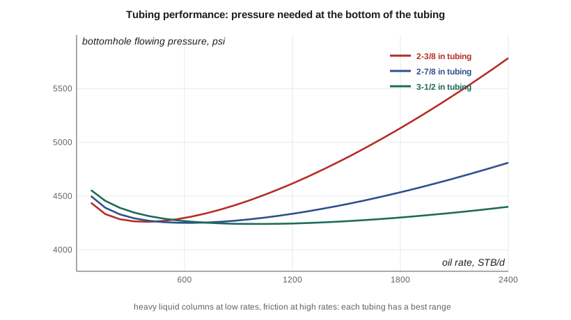

Reading the outflow curve

Every outflow curve has the same shape. At very low rates, slip is large, liquid accumulates, and the column is heavy, so a high bottomhole pressure is needed. As the rate rises, slip falls and the column becomes lighter, so the required pressure falls. At high rates, friction takes over and the required pressure rises again. The minimum of the curve marks the rate at which the tubing works best. To the left of the minimum, flow is unstable: a small drop in rate makes the column heavier, which reduces the rate further, and the well tends to load up and die or to flow in heads.

The results for the 4-22H show this clearly. At its current 1,050 STB/d, the 2-7/8 in tubing needs about 4,300 psi at the bottom, while 3-1/2 in tubing would need about 4,240 psi and 2-3/8 in about 4,520 psi, because friction is already significant at this rate. At 250 to 500 STB/d, the smaller tubing becomes the best choice. At 100 STB/d, all three sizes need about 4,400 to 4,500 psi. The well is near the minimum of its 2-7/8 in curve, and as its rate falls it will move onto the unstable side where smaller tubing would help.

The lesson for tubing selection is that there is no single correct size. Large tubing suits high rates early in life; small tubing suits low rates later. Some operators run large tubing first and replace it with smaller tubing or a velocity string later; others choose a compromise size. For wells that will go on artificial lift soon anyway, the tubing must also suit the lift method: rod pumps need tubing large enough for the pump and rods, and gas lift needs mandrels for the valves.

What changes the outflow curve

Several well parameters shift the outflow curve up or down. Higher wellhead pressure adds directly to the required bottomhole pressure, and more than one for one at low rates because it also compresses the gas. Higher water cut makes the column heavier and moves the whole curve up; this is the main reason wells stop flowing as they age. Higher gas-liquid ratio lightens the column and moves the curve down, up to a point beyond which friction from the extra gas outweighs the benefit. Greater depth raises the curve in proportion. Finally, temperature affects gas volume and fluid viscosity, and for waxy crudes, falling temperature can deposit paraffin that narrows the tubing over time.