Water drive and aquifer models

While the Bakken unit shows no aquifer support, Lena wants Ethan to learn the methods on a pool that does. 'The company also owns part of the Mission Canyon pool, a conventional carbonate reservoir under the east side of the field,' she says. 'It has an edge aquifer and five years of history. If we ever waterflood anything, or buy a pool like it, you need to know how to recognize water drive and size the aquifer.'

Many oil and gas reservoirs are bounded by water-bearing rock, the aquifer, which is part of the same porous layer. When reservoir pressure falls, the aquifer water expands and the aquifer rock compacts, and water flows into the reservoir, replacing produced fluids and supporting pressure. This lesson describes water drive, the main analytical aquifer models, and how to detect and size an aquifer with the material balance.

How water drive works

Water and rock are only slightly compressible, so a small aquifer supplies little energy. But aquifers can be very large, many times the volume of the reservoir, and some are connected to an outcrop where surface water recharges them. A large, permeable aquifer can maintain reservoir pressure almost completely; a small or tight one helps only a little. Engineers describe aquifers by their size, their permeability and their geometry relative to the reservoir.

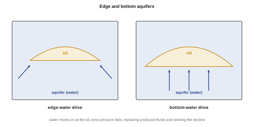
In edge-water drive the aquifer lies around the flanks of the reservoir and water advances laterally, reaching the down-dip wells first. In bottom-water drive the oil sits on top of water across the whole reservoir, and water rises vertically; wells in such reservoirs are prone to water coning, where the pressure drawdown pulls water upward into the well.

A strong water drive gives a distinctive history: pressure stays high, the gas-oil ratio stays near the solution value because the pressure never falls far below the bubble point, and water production begins early in down-dip wells and rises steadily. Recovery is high, often 35 to 60 percent of the oil in place, because water sweeps the oil much like a natural waterflood. Weak water drive gives behavior between solution-gas drive and full pressure support.

Aquifer models

Because the aquifer is rarely drilled, its properties are not measured directly. Instead, engineers choose a mathematical model of water influx and adjust its parameters until the material balance matches the observed pressure history. Three models are common.

The pot aquifer is the simplest. It assumes the aquifer is small and permeable enough that its pressure equals the reservoir pressure at all times. Influx is then just the expansion of the aquifer water and rock.

Here Wi is the initial aquifer water volume. Because the pot model's influx is proportional to the pressure drop, just like the reservoir's own expansion terms, it cannot be distinguished from a larger reservoir in a material balance fit; the two trade off against each other. It is useful mainly for small aquifers.

Schilthuis's steady-state model assumes the aquifer is so large and permeable that its outer pressure stays at the initial value, so that influx rate is proportional to the pressure difference between the aquifer and the reservoir boundary. Cumulative influx is then the time integral of the pressure drop.

The constant k' is the influx constant. Because influx in this model depends on how long the pressure has been depressed, not just how far, it behaves differently from the reservoir's expansion terms and can be separated from them in a material balance fit.

The van Everdingen-Hurst unsteady-state model treats the aquifer as a radial or linear body of finite or infinite size and solves the diffusivity equation for flow within it (lesson 10). Influx depends on the whole pressure history, through superposition of the solutions for each pressure step. It is the most rigorous of the classical models but needs dimensionless influx tables or numerical evaluation. Fetkovich's method approximates the unsteady behavior with a pseudosteady-state aquifer of finite size, and is widely used because it is simple to compute and reasonably accurate for most aquifers. Modern simulators include these models as boundary conditions.

Detecting and sizing water influx with material balance

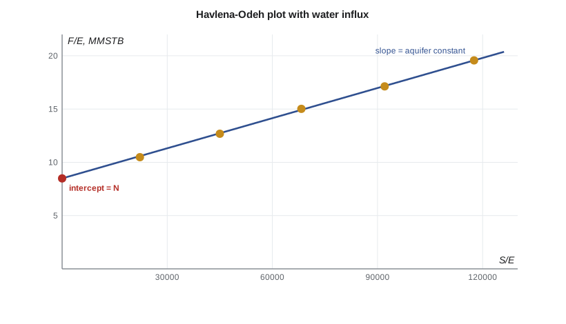
With water influx included, the material balance for an undersaturated reservoir without a gas cap becomes F = N (Eo + Efw) + We Bw. If the influx follows Schilthuis's model, We = k' S, where S is the running integral of the pressure drop over time. Dividing by the expansion term E = Eo + Efw gives a straight line.

A plot of F/E against S/E is a straight line with intercept N and slope k' if the model is right. If the points curve upward, the aquifer is stronger than the steady-state model assumes or the influx model is wrong in form; if they curve downward, it is weaker. Engineers try several aquifer models and choose the one that gives the straightest line and a physically reasonable aquifer size.

# Detecting and sizing water influx: Havlena-Odeh with a Schilthuis steady-state aquifer and a pot aquifer
import math
SI = False  
if SI:   # yearly pressures (kPa) and cumulative oil (m3) for the oil pool, from lesson 5
    p_hist = [15300, 15050, 14800, 14550, 14300, 14090]
    Np = [0.0, 4210.0, 8890.0, 14220.0, 19730.0, 25460.0]
    to_psi = lambda p: p / 6.895
    pb, bob, co, cf, cw, swc, scale, unit = 1856.0, 1.300, 1.4e-5, 4.21e-6, 3.0e-6, 0.30, 1e6, "10^6 m3"
else:    # yearly pressures (psia) and cumulative oil (STB) for the conventional pool
    p_hist = [3150, 3060, 2975, 2895, 2820, 2755]
    Np = [0.0, 17900.0, 42100.0, 72600.0, 107100.0, 146400.0]
    to_psi = lambda p: p
    pb, bob, co, cf, cw, swc, scale, unit = 1450.0, 1.21, 1.2e-5, 4.5e-6, 3.0e-6, 0.25, 1e6, "MMSTB"
bo = lambda p: bob * math.exp(-co * (to_psi(p) - pb))
boi = bo(p_hist[0])
F, E, S, D = [], [], [], []
s = 0.0
for j in range(1, len(p_hist)):
    p = p_hist[j]; dp = p_hist[0] - p
    s += p_hist[0] - (p_hist[j] + p_hist[j - 1]) / 2          # Schilthuis: integral of pressure drop over time (1-year steps)
    F.append(Np[j] * bo(p))
    E.append(bo(p) - boi + boi * (cw * swc + cf) / (1 - swc) * to_psi(dp))
    S.append(s); D.append(dp)
def fit2(x1, x2, y):          # least squares y = a*x1 + b*x2
    s11 = sum(a * a for a in x1); s22 = sum(b * b for b in x2); s12 = sum(a * b for a, b in zip(x1, x2))
    s1y = sum(a * c for a, c in zip(x1, y)); s2y = sum(b * c for b, c in zip(x2, y))
    det = s11 * s22 - s12 * s12
    a = (s1y * s22 - s2y * s12) / det; b = (s2y * s11 - s1y * s12) / det
    rms = math.sqrt(sum((a * u + b * v - c) ** 2 for u, v, c in zip(x1, x2, y)) / len(y))
    return a, b, rms
vu, ku = ("m3", "m3 per kPa per year") if SI else ("rb", "rb per psi per year")
N0 = sum(f * e for f, e in zip(F, E)) / sum(e * e for e in E)
rms0 = math.sqrt(sum((N0 * e - f) ** 2 for e, f in zip(E, F)) / len(F))
print(f"no aquifer (volumetric)  : N = {N0/scale:5.2f} {unit}, rms misfit {rms0:7.0f} {vu}")
N, k, rms = fit2(E, S, F)
print(f"Schilthuis steady-state  : N = {N/scale:5.2f} {unit}, aquifer constant {k:.2f} {ku}, rms misfit {rms:5.0f} {vu}")
print("Havlena-Odeh check, F/E against S/E:")
for f, e, x in zip(F, E, S):
    print(f"   S/E = {x/e:12,.0f}   F/E = {f/e/scale:6.2f} {unit}")
we = k * S[-1]
print(f"water influx to date {we:,.0f} {vu}, {we/F[-1]:.0%} of the reservoir withdrawal")

no aquifer (volumetric)  : N = 17.27 MMSTB, rms misfit   14879 rb
Schilthuis steady-state  : N =  8.49 MMSTB, aquifer constant 94.23 rb per psi per year, rms misfit   297 rb
Havlena-Odeh check, F/E against S/E:
   S/E =       22,189   F/E =  10.48 MMSTB
   S/E =       44,998   F/E =  12.68 MMSTB
   S/E =       68,265   F/E =  15.02 MMSTB
   S/E =       92,035   F/E =  17.13 MMSTB
   S/E =      117,551   F/E =  19.57 MMSTB
water influx to date 98,711 rb, 57% of the reservoir withdrawal

For the Mission Canyon pool, the no-aquifer fit leaves a systematic misfit of about 15,000 rb and an apparent oil in place of 17 MMSTB, double the volumetric value, while the Schilthuis fit reduces the misfit to about 300 rb and gives N = 8.49 MMSTB, close to the maps. The aquifer constant is about 94 rb per psi per year, and water influx to date is about 99,000 rb, more than half of the reservoir withdrawal. Lena summarizes: a moderately strong edge aquifer, which explains why the pool's down-dip wells began producing water in their third year and why its pressure has fallen only 400 psi.

Water production and coning

Water drive brings water with it. As the water advances, wells cut more water, and the cost of lifting, separating, treating and disposing of it rises. In edge-water reservoirs, down-dip wells water out first and are often converted to water injectors or shut in. In bottom-water reservoirs, water coning limits the rate at which wells can produce without drawing water up: above a critical rate, the cone breaks through and the water cut rises sharply. Horizontal wells, placed high in the oil column, reduce coning because they spread the drawdown along their length.

Water production also gives information. The timing of water breakthrough at each well and the rise of water cut help locate the advancing front and calibrate the aquifer model. Produced water chemistry can distinguish formation water from injected water.

Aquifers in gas reservoirs

Water influx affects gas reservoirs too, and often more harmfully. Water advancing into a gas reservoir traps gas behind it at a high residual gas saturation, often 20 to 35 percent of pore volume, and it can water out wells while much gas remains. As a result, recovery from water-drive gas reservoirs is often lower than from volumetric ones, sometimes 50 to 70 percent instead of 80 to 90. The p/z plot of lesson 8 is the main tool for detecting such influx.

Using the aquifer model

Once calibrated, the aquifer model becomes part of every forecast. It tells the engineer how much pressure support to expect at higher production rates, how much water will be produced, and how much injection a waterflood would need to supplement the natural support. Because aquifer parameters come from history matching rather than direct measurement, their uncertainty should be carried into the forecasts by running cases with weaker and stronger aquifers that still match the history acceptably.

Choosing among aquifer models

In practice, several aquifer models can match the same pressure history almost equally well, especially when the history is short. The choice should then rest on geology as well as statistics: the mapped extent of the water leg, its permeability from water-bearing wells or tests, and evidence of an outcrop or recharge. Engineers also prefer the simplest model that matches, then test the forecast with the alternatives. A forecast that changes greatly between acceptable aquifer models tells the team that more data, such as a pressure gauge in an aquifer well, would be valuable before a large decision is made.