The general material balance equation

Lena puts the study unit's production and pressure history on the table: cumulative oil from the 3-22H well and its sister well, with average reservoir pressures estimated from shut-in buildups and downhole gauges. 'Volumetrics told us what the maps say,' she says. 'Material balance tells us what the reservoir says. It doesn't care about our maps. It only asks how much pressure we lost for each barrel we took out. If the two answers disagree, the reservoir is trying to tell us something.'

The material balance equation is the reservoir engineer's most fundamental tool. It states that the reservoir volume of fluids removed from a reservoir equals the expansion of the fluids and rock left behind plus any fluids that have entered. It treats the reservoir as a single tank at one average pressure, so it ignores where in the reservoir things happen, but it captures the volumes and energy exactly. This lesson builds the general equation, rearranges it into the straight-line form of Havlena and Odeh, and applies it to the pool above its bubble point.

The tank model and its assumptions

Material balance assumes that the reservoir behaves as one tank, with uniform pressure throughout at any time, and that the PVT properties at that average pressure apply everywhere. In practice pressure varies across a reservoir while wells are producing, so the method uses volume-weighted average reservoir pressures, usually from shut-in pressure tests. The tank assumption works well when permeability is high enough for pressure to equalize between surveys; in tight reservoirs, where pressure differences persist, the method describes only the volume the wells are draining and must be used with care.

Material balance also needs reliable cumulative production of oil, gas and water, the volumes of any injected fluids, and the PVT data of lesson 3. Its inputs are mostly measured routinely in the field, which is its great advantage: it gives an independent estimate of oil in place from data that would be collected anyway.

Building the equation

Consider a reservoir with N stock-tank volumes of oil initially, a gas cap whose reservoir volume is m times the initial oil zone volume, and an aquifer. When the average pressure falls from pi to p, the following volumes, all at reservoir conditions, must balance. On the withdrawal side: the produced oil Np with its share of produced gas, and the produced water Wp. On the expansion side: the oil and its originally dissolved gas, the gas cap gas, the connate water and the pore volume, plus water influx We from the aquifer and any injected water or gas.

Writing each term in reservoir volumes gives the general material balance equation. The withdrawal term F uses the total formation volume factor Bt and the cumulative produced gas-oil ratio Rp = Gp/Np, so that all produced gas, whether it came from solution or from the gas cap, is accounted for.

The expansion terms are written per stock-tank volume of initial oil, so that each is multiplied by N.

Here Eo is the expansion of the oil and its dissolved gas, Eg the expansion of the gas cap, and Efw the expansion of connate water and the reduction in pore volume, with Δp = pi − p. Above the bubble point, Bt equals Bo and Rp equals Rsi, so the produced gas term disappears and Eo is simply Bo − Boi. Putting the pieces together:

The Havlena-Odeh straight line

Havlena and Odeh observed in the 1960s that the material balance equation, written this way, is a straight line in suitable variables, and that plotting it shows at once whether the assumptions are right. For the simplest case, an undersaturated reservoir with no gas cap and no water influx, the equation reduces to F = N (Eo + Efw). A plot of F against Eo + Efw should then be a straight line through the origin with slope N.

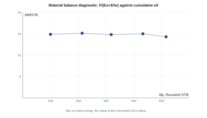
A second, more sensitive plot divides through: F/(Eo + Efw) against cumulative production or time. If the assumptions are right, it is a horizontal line at the value N. Its shape is a diagnosis. A line that rises with time means an extra energy source is helping, usually an aquifer, so the simple equation overestimates N. A line that falls means less energy than assumed, for example because the expansion terms are overstated, the pressures are too low, or part of the reservoir is not connected. Lena calls it 'the plot that keeps us honest.'

Applying it above the bubble point

For the study unit, all the history is above the bubble point and there is no gas cap, so Eg drops out. The produced water is mostly fracturing fluid returning early in each well's life, and Lena asks Ethan to leave it out of this first pass and test its effect later. No fluids have been injected. Ethan calculates F and Eo + Efw at each pressure estimate, using the Bo function from lesson 3 and the compressibilities from lesson 4.

# Havlena-Odeh material balance for an undersaturated oil reservoir: F = N (Eo + Efw)
import math
SI = False  
if SI:   # pressure kPa, cumulative oil m3 (no water produced, no injection, no aquifer)
    hist = [(15300, 0.0), (15050, 4210.0), (14800, 8890.0), (14550, 14220.0), (14300, 19730.0), (14090, 25460.0)]
    to_psi = lambda p: p / 6.895
    pb, bob, co, cf, cw, swc = 1856.0, 1.300, 1.4e-5, 4.21e-6, 3.0e-6, 0.30
    unit, scale = "10^6 m3", 1e6
else:    # pressure psia, cumulative oil STB
    hist = [(5370, 0.0), (5100, 99900.0), (4800, 213800.0), (4500, 318500.0), (4200, 432600.0), (3900, 516300.0)]
    to_psi = lambda p: p
    pb, bob, co, cf, cw, swc = 2600.0, 1.518, 1.5e-5, 5.39e-6, 3.0e-6, 0.35
    unit, scale = "MMSTB", 1e6
bo = lambda p: bob * math.exp(-co * (p - pb))      # above the bubble point only
pi = to_psi(hist[0][0]); boi = bo(pi)
rows = []
for P, Np in hist[1:]:
    p = to_psi(P); dp = pi - p
    F = Np * bo(p)                                  # reservoir volume withdrawn
    Eo = bo(p) - boi                                # oil expansion per unit of oil in place
    Efw = boi * (cw * swc + cf) / (1 - swc) * dp    # connate water and pore volume change
    rows.append((P, F, Eo + Efw, F / (Eo + Efw)))
print(" pressure        F         Eo+Efw        F/(Eo+Efw)")
for P, F, E, n in rows:
    print(f" {P:7,.0f}  {F:11,.0f}  {E:12.6f}  {n/scale:9.2f} {unit}")
N = sum(F * E for _, F, E, _ in rows) / sum(E * E for _, _, E, _ in rows)   # least squares line through the origin
print(f"slope of F against (Eo+Efw), forced through the origin: N = {N/scale:.2f} {unit}")
print(f"recovery to date: {hist[-1][1]/N:.2%} of that oil in place")
trend = rows[-1][3] / rows[0][3]
print("F/(Eo+Efw) " + ("rises steadily with time: an extra energy source (lesson 7) is likely" if trend > 1.1 else "is roughly constant: no sign of extra energy"))

 pressure        F         Eo+Efw        F/(Eo+Efw)
   5,100      146,067      0.009805      14.90 MMSTB
   4,800      314,013      0.020728      15.15 MMSTB
   4,500      469,898      0.031680      14.83 MMSTB
   4,200      641,114      0.042663      15.03 MMSTB
   3,900      768,608      0.053675      14.32 MMSTB
slope of F against (Eo+Efw), forced through the origin: N = 14.68 MMSTB
recovery to date: 3.52% of that oil in place
F/(Eo+Efw) is roughly constant: no sign of extra energy

The result is reassuring. F/(Eo + Efw) stays close to 15 MMSTB, with no trend beyond the scatter expected from estimated average pressures, and the line through the origin gives 14.68 MMSTB, close to the volumetric P50 of 15.19 MMSTB. The flat trend says that no extra energy source is acting, as expected in the tight Bakken with no connected aquifer. Lena points out one caution: in such tight rock, material balance measures the oil connected to the wells over the time of the history, which can grow as the pressure disturbance spreads, so the value should be updated as more data arrive.

Sensitivity and data quality

Material balance is sensitive to average pressure. In an undersaturated reservoir the expansion terms are small, so a small error in pressure is a large error in Eo + Efw and therefore in N. Early in a reservoir's life, when the pressure drop is only a few percent of the initial pressure, material balance estimates can be wildly wrong. A common rule of thumb is to wait until 5 to 10 percent of the initial pressure has been depleted, or a few percent of the oil produced, before trusting the result. Even then, engineers test the sensitivity by varying the pressures within their uncertainty.

Average pressure itself is an estimate. It comes from buildup tests, static gradients or downhole gauges, corrected to a common datum depth, and weighted by the volume each well drains. Errors in the datum correction, in the extrapolation of buildups or in the weights all flow straight into the result. In tight reservoirs, where buildups take months to reach the average pressure, the estimates may be poor; this is one reason material balance is used with caution in shale and tight oil.

Cumulative production must be accurate too. Allocated production from shared facilities, unmeasured gas and early unrecorded volumes can all bias F. Engineers compare the material balance with metered sales and with well tests to catch such errors.

Uses of material balance

Beyond estimating oil in place, the material balance has three other main uses. It identifies the drive mechanisms acting in a reservoir and their relative importance, through drive indices (lesson 6). It estimates aquifer size and strength by matching pressure history (lesson 7). And, once the reservoir is characterized, it predicts future pressure for a planned production schedule, which tells the engineer, for example, when the bubble point will be reached or how much injection is needed to hold pressure.

Material balance is also the backbone of reservoir simulation: every simulator cell obeys it, and a simulation model that does not reproduce a field-wide material balance is wrong. Experienced engineers often run a material balance before building a simulation model, because it quickly reveals data problems and the drive mechanisms the model must capture.

Predicting pressure with the material balance

Once N and the drive terms are known, the material balance can be run forward. For a planned production schedule, the engineer guesses the pressure at the end of each period, calculates the expansion terms and any influx at that pressure, and adjusts the guess until the withdrawal equals the expansion plus influx. Above the bubble point this is a simple calculation; below it, the gas-oil ratio must also be predicted, which is the subject of lesson 6. The result is a pressure forecast that shows, for example, how many months remain before the bubble point is reached at a higher production rate, which is often the deciding factor in when to start pressure maintenance.

Ethan runs that forecast for the higher rates that more horizontal wells would bring. The answer is sobering: at the doubled rate, the pool would reach its bubble point within about two years. Lena circles the result. 'That date,' she says, 'is the real deadline for the waterflood decision.'