Transient and pseudosteady-state radial flow

Ethan's steady-state analysis assumed the pressure at the edge of the drainage area stays constant. 'In most reservoirs it doesn't,' Lena says. 'When a well starts, the pressure disturbance spreads out from it, reaches the edges of its drainage area, and then the whole area depletes together. In the Bakken, the disturbance spreads so slowly that the wells may stay in the first stage for years. The equations for those stages are what well tests and decline curves are built on.'

This lesson introduces the diffusivity equation, which governs how pressure changes with time and distance in a reservoir, and its solutions for a well producing at constant rate: infinite-acting transient flow, the radius of investigation, and pseudosteady state. It lays the groundwork for well test analysis in PET-360 and for decline analysis in lesson 12.

The diffusivity equation

Combining Darcy's law with conservation of mass and the compressibility of a slightly compressible fluid gives the radial diffusivity equation. It is the same equation that describes heat conduction (MEC-340), with pressure in place of temperature.

Here ct is the total compressibility, the saturation-weighted sum of the fluid and pore compressibilities, and the group k/(φ μ ct) is the hydraulic diffusivity. It measures how fast a pressure change travels through the rock: high permeability and low compressibility spread it quickly, tight rock and viscous fluid slowly. The equation assumes a homogeneous, isotropic reservoir of uniform thickness, a single slightly compressible fluid and small pressure gradients. Gas flow uses pseudopressure and pseudotime to satisfy those assumptions approximately.

Infinite-acting flow: the line-source solution

When a well starts producing at constant rate from a reservoir at uniform initial pressure, the pressure disturbance spreads outward. Until it reaches a boundary, the reservoir behaves as if it were infinite. Treating the well as a line of zero radius, the solution is the exponential integral, often called the line-source or Theis solution, after the hydrologist who used it for water wells in 1935.

E1 is the exponential integral function, written in some texts as −Ei(−x). For small arguments, which applies at the wellbore after a short time, it is well approximated by −0.5772 − ln x. The pressure at the well then falls in proportion to the logarithm of time.

This logarithmic behavior is the basis of the semilog analysis of well tests. A plot of flowing pressure against the logarithm of time is a straight line whose slope is inversely proportional to kh. From the slope, an engineer obtains the permeability, and from the position of the line, the skin. The same idea, applied to a pressure buildup after shut-in, is Horner's method, the most widely used well test analysis.

Radius of investigation

The pressure disturbance spreads with the square root of time. A convenient measure is the radius of investigation, the distance at which the pressure change reaches a fixed small fraction of the change at the well. One common definition, in oilfield units with time in hours, is shown below; in consistent SI units the equivalent is about 2√(k t/(φ μ ct)).

The radius of investigation matters in two ways. In well testing it sets how far into the reservoir a test sees: a short test in tight rock investigates only the rock near the well. In development planning it sets when a well begins to feel its neighbors or its boundaries, and so when its decline will steepen.

Pseudosteady state

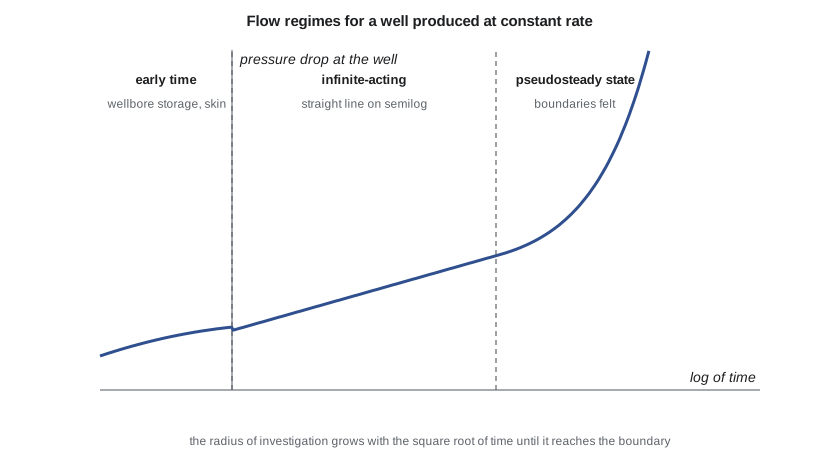
Once the pressure disturbance reaches all the no-flow boundaries of the well's drainage area, whether real faults or the dividing lines between neighboring wells, the flow enters pseudosteady state. The pressure everywhere in the drainage area then declines at the same constant rate, and the shape of the pressure profile stays fixed. The rate of decline follows directly from material balance on the drainage volume: the produced reservoir volume equals ct times the pore volume times the pressure drop.

The inflow equation in pseudosteady state is like the steady-state equation, but it uses the average reservoir pressure and a slightly different constant.

For drainage areas that are not circular, or wells not at the center, Dietz's shape factors replace the 0.75 term. Pseudosteady-state flow is the basis of the productivity index used in forecasting, of reservoir limit tests that estimate the drainage volume from the rate of pressure decline, and of the exponential decline that a well at constant flowing pressure shows once it is boundary-dominated (lesson 12).

From transient to boundary-dominated

Every well passes through these regimes. Right after it starts, wellbore storage and skin dominate the first minutes or hours. Then comes the infinite-acting period, which can last hours in a permeable reservoir or years in a tight one. Finally boundary-dominated flow begins. Which regime a well is in determines which analysis is valid. Applying a boundary-dominated method, such as conventional decline curves or material balance, to a well still in transient flow gives misleading results, a common error in tight reservoirs.

# Transient (line-source) and pseudosteady-state radial flow; radius of investigation
import math
SI = False  
def E1(x):        # exponential integral E1(x) = -Ei(-x), series for small x and continued fraction for large x
    if x < 1.0:
        s, term, n = -0.5772156649 - math.log(x), 1.0, 1
        while True:
            term *= -x / n; add = -term / n; s += add; n += 1
            if abs(add) < 1e-12: return s
    f = 0.0
    for n in range(60, 0, -1): f = n / (1 + n / (x + f))
    return math.exp(-x) / (x + f)
# calculations in oilfield units; the ca site converts the inputs and the printed results
if SI:
    k, h, phi, mu, ct, B, q, rw, re, pi, s = 15.0, 6.5 / 0.3048, 0.14, 0.72, 1.49e-5, 1.29, 37.3 * 6.29, 0.10 / 0.3048, 400 / 0.3048, 15300 / 6.895, 0.0
    P = lambda p: f"{p*6.895:8,.0f} kPa"; L = lambda r: f"{r*0.3048:7,.0f} m"
else:
    k, h, phi, mu, ct, B, q, rw, re, pi, s = 25.0, 30.0, 0.12, 0.90, 1.6e-5, 1.19, 475.0, 0.354, 1490.0, 3150.0, 0.0
    P = lambda p: f"{p:7,.0f} psia"; L = lambda r: f"{r:6,.0f} ft"
print("time        flowing pressure    radius of investigation")
for t in (0.5, 2, 10, 50, 150):                                # hours, while the well is still infinite-acting
    x = 948 * phi * mu * ct * rw ** 2 / (k * t)
    pwf = pi - 70.6 * q * B * mu / (k * h) * (E1(x) + 2 * s)
    ri = math.sqrt(k * t / (948 * phi * mu * ct))
    print(f"{t:6.1f} h  {P(pwf)}        {L(ri)}")
t_bound = 948 * phi * mu * ct * re ** 2 / k
print(f"radius of investigation reaches the drainage boundary after about {t_bound:,.0f} h ({t_bound/24:,.0f} days)")
pbar = pi - (1000 / 6.895 if SI else 150.0)                    # average pressure after some depletion (assumed)
pwf_pss = pbar - q * mu * B * (math.log(re / rw) - 0.75 + s) / (0.00708 * k * h)
print(f"pseudosteady state: average pressure {P(pbar).strip()}, flowing pressure {P(pwf_pss).strip()}")
kt = 0.01 if SI else 0.005
print(f"in {kt} mD tight rock the same well investigates only {L(math.sqrt(kt * 8760 / (948 * phi * mu * ct))).strip()} in a year")

time        flowing pressure    radius of investigation
   0.5 h    2,650 psia            87 ft
   2.0 h    2,584 psia           175 ft
  10.0 h    2,507 psia           391 ft
  50.0 h    2,430 psia           874 ft
 150.0 h    2,377 psia         1,513 ft
radius of investigation reaches the drainage boundary after about 145 h (6 days)
pseudosteady state: average pressure 3,000 psia, flowing pressure 2,272 psia
in 0.005 mD tight rock the same well investigates only 164 ft in a year

For the Mission Canyon vertical well, the infinite-acting period ends after about six days: the radius of investigation reaches the 1,490 ft drainage radius in about 145 hours. After that, the well is in pseudosteady state. In 0.005 mD rock like the Bakken, the same well would investigate only about 160 ft in a whole year. Fractured horizontal wells in the Bakken are therefore in transient linear flow toward their fractures for months to years, which is why their declines are so steep and why their decline exponents exceed one (lesson 12).

Superposition

Because the diffusivity equation is linear, solutions can be added. Superposition in time handles rate changes: a well whose rate changes from q1 to q2 behaves as if a second well, producing q2 − q1, started at the moment of the change. A shut-in is the special case where q2 is zero, which is the basis of buildup test analysis. Superposition in space handles several wells interfering with each other, and image wells represent straight boundaries such as sealing faults. These ideas underlie most well test interpretation and many quick reservoir calculations.

Using these concepts in the study

For the study, Ethan uses these ideas to judge the pressure estimates used in the material balance. The buildups in the Bakken wells never reached radial flow, so their average pressures came from rate-transient analysis rather than from simple extrapolation, and Lena widens the uncertainty band on them accordingly. He also notes that the 3-22H well's decline exponent of about 1.2 is consistent with long transient linear flow, an important point for the forecast in lesson 12.

Dimensionless variables

Reservoir engineers often write the diffusivity equation and its solutions in dimensionless form. Dimensionless pressure pD scales the pressure drop by the group q μ B/(2π k h); dimensionless time tD scales time by the diffusivity and the wellbore radius squared; and dimensionless radius rD is r/rw. In these variables, the line-source solution becomes pD = ½ E1(rD²/(4 tD)), the same for every reservoir. Dimensionless solutions can then be tabulated or plotted once and reused, which is how type curves for well test and decline analysis are built. Converting a field problem to dimensionless form, reading the solution, and converting back is a routine skill in PET-360.

Interference between wells

When two wells produce from the same reservoir, each feels the other once their radii of investigation overlap. By superposition, the pressure drop at one well is its own drop plus the drop caused at its location by the other well. Interference tests use this deliberately: one well is produced or injected while a nearby observation well records the small pressure response, which gives the permeability and storage of the rock between them.

For the study, Ethan notes that the Mission Canyon wells are far enough apart that their interference only began after several months, which is consistent with their pressure surveys showing slightly different values early in the pool's life and almost identical values later. In the Bakken unit, by contrast, the two horizontal wells may take years to interfere.