
NUC-440 · Lesson 1 of 12 · 21 min
Control system principles
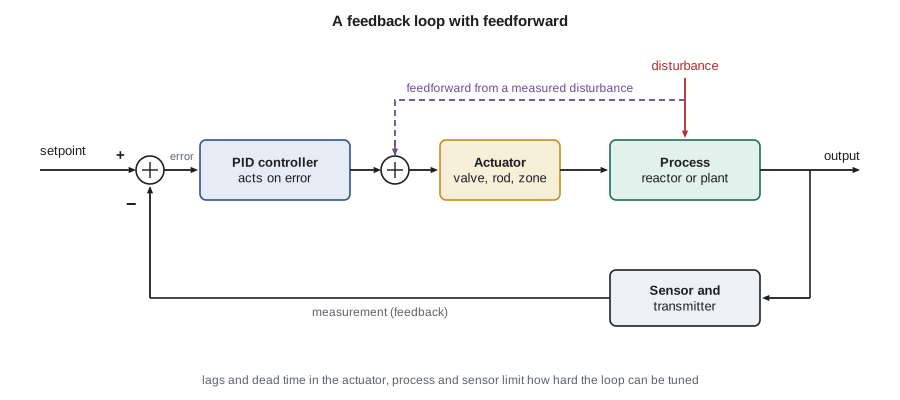
Hana Okoye's next rotation at Meridian Nuclear Engineering in Knoxville is with the instrumentation and control group, the engineers who look after the sensors, controllers, computers and protection logic for TVA's pressurized water reactor fleet and for the BWRX-300 project at Clinch River. The group lead, Andrea Kowalczyk, started her career commissioning a digital feedwater control upgrade at a Westinghouse four-loop plant, and she begins Hana's first morning with a sketch on a whiteboard: a box labeled plant, an arrow labeled measurement coming out of it, a circle where the measurement is compared with a setpoint, and a box labeled controller that drives a valve or a rod back into the plant. “Everything we do in this group is a version of this loop,” she says. “Rod control, pressurizer pressure, steam generator level, even the reactor protection system, which is a loop that only ever acts once. If you understand the loop, you can learn any system in the plant.”
This lesson sets out the vocabulary of control that the rest of the course uses. It reviews feedback and feedforward, the proportional, integral and derivative actions, dead time and lags, stability and tuning, cascade and ratio control, and the way control functions are separated from protection functions in a nuclear plant. Most of this material will be familiar from a general control course; the emphasis here is on why each idea matters in a reactor.
Open loop and closed loop
An open-loop controller sets its output without looking at the result. A toaster timer is open loop: it heats for a fixed time whether the bread is pale or burnt. A closed-loop, or feedback, controller measures the controlled variable, compares it with the desired value, and adjusts its output to reduce the difference. The desired value is the setpoint, the difference is the error, the thing the controller adjusts is the manipulated variable, and everything that pushes the controlled variable away from the setpoint without the controller's help is a disturbance.
Feedback has three great virtues. It corrects for disturbances that nobody predicted, it reduces the effect of uncertainty in the plant, and it can make a slow or unstable plant behave quickly and stably. It has one great weakness: it can only act after an error has appeared, and if the loop is too aggressive it can make matters worse by overcorrecting. Most of the art of control engineering lies in getting the benefits of feedback without its weakness.
Proportional, integral and derivative action
The most widely used controller combines three actions. Proportional action makes the output proportional to the present error: a large error gives a large correction. On its own it leaves a steady offset, because some error is needed to hold the output away from its resting value. Integral action adds a term proportional to the accumulated error, so the output keeps moving until the error is exactly zero; it removes offset but adds phase lag that can cause overshoot. Derivative action adds a term proportional to the rate of change of the error, anticipating where the error is going; it can damp a loop but amplifies measurement noise, so it is used sparingly on noisy signals such as flow and neutron flux.
Here u is the controller output, e is the error, K_c is the controller gain, T_i is the integral or reset time and T_d is the derivative time. In practice the output is limited by the range of the actuator, so a practical controller also needs protection against integral windup: when the output is saturated, the integral term must stop accumulating, or the controller will hold the actuator against its limit long after the error has reversed. The digital controllers in a modern plant also filter the measured signal, apply rate limits to the output, and switch between automatic and manual without a bump in the output.
Lags, dead time and the plant's character
Every real loop contains delays. A thermal process such as a fuel element or a steam generator tube bundle stores energy and responds with a lag: after a step change in input, its output rises along an exponential curve whose time constant is the stored energy divided by the rate at which energy can flow. A measurement may add its own lag, such as the time for a thermowell to warm a resistance thermometer. Transport delay, or dead time, is different: nothing at all happens until a fluid packet travels from the point of change to the sensor. In a primary heat transport loop, the time for coolant to travel from the core outlet to a hot-leg temperature sensor is a few seconds; the time for a change in feedwater temperature to reach the reactor inlet is longer.
Dead time is the enemy of tight control. A controller cannot correct an error it has not yet seen, and if it acts strongly on old information, it overcorrects. The ratio of dead time to the dominant time constant is the single best guide to how hard a loop can be pushed. Loops with small ratios, such as most pressure loops, can be tuned tightly; loops with large ratios need gentle tuning or a model-based structure that predicts the effect of the delay.
# PI control of a first-order process with dead time: compare three tunings.
def simulate(kc, ti, K=2.0, tau=20.0, dead=4.0, dt=0.1, t_end=300.0):
    n_dead = int(dead / dt); buf = [0.0] * n_dead
    y = integ = 0.0; sp = 1.0; out = []; peak = 0.0; settle = None
    for k in range(int(t_end / dt)):
        t = k * dt
        e = sp - y
        integ += e * dt
        u = kc * (e + integ / ti)
        u = max(-5.0, min(5.0, u))          # actuator limits
        buf.append(u); u_late = buf.pop(0)    # transport delay
        y += dt * (K * u_late - y) / tau      # first-order lag
        peak = max(peak, y)
        if abs(y - sp) > 0.02: settle = None
        elif settle is None: settle = t
        out.append(y)
    return peak, settle, out[-1]
print(f"{'tuning':22s}{'Kc':>6s}{'Ti (s)':>8s}{'overshoot':>11s}{'settle (s)':>12s}")
for name, kc, ti in [("sluggish", 0.4, 30.0), ("moderate", 1.0, 20.0), ("aggressive", 2.2, 8.0)]:
    peak, ts, yf = simulate(kc, ti)
    ts_txt = f"{ts:12.1f}" if ts is not None else f"{'none':>12s}"
print(f"{name:22s}{kc:6.1f}{ti:8.1f}{max(0.0, peak - 1) * 100:10.1f}%{ts_txt}")tuning Kc Ti (s) overshoot settle (s) sluggish 0.4 30.0 0.0% 172.9 moderate 1.0 20.0 0.0% 21.3 aggressive 2.2 8.0 82.8% 83.1
The output shows the trade-off. The sluggish tuning never overshoots but takes almost three minutes to settle. The moderate tuning reaches the setpoint in about twenty seconds without overshoot. The aggressive tuning, with high gain and a short integral time, overshoots by more than 80 percent and rings for over a minute before it settles, because it acts hard on information that is four seconds old. Andrea points out that in a nuclear plant a tuning that rings is worse than slow: oscillating flows and temperatures cycle the equipment, confuse the operators, and can take a process variable toward a trip setpoint.
Stability and tuning
A loop is stable if a disturbance dies away rather than growing. Stability can be analyzed in the frequency domain with Bode or Nyquist plots, or in the time domain with step responses. Two margins are commonly quoted. The gain margin is the factor by which the loop gain could increase before the loop became unstable; the phase margin is the additional phase lag the loop could tolerate at the frequency where the loop gain is one. Margins of around a factor of two in gain and 45 degrees in phase are typical targets for plant loops, leaving room for changes in the plant as conditions change.
Plant characteristics do change. The gain of a feedwater valve depends on the pressure drop across it. The reactivity worth of a control device depends on the flux shape and the burnup of the surrounding fuel. The response of reactor power to reactivity depends on power level because the temperature feedbacks change. Controllers are therefore often gain-scheduled, with gains that vary with power or flow, and they are tuned and retested during commissioning at several power levels. Standard tuning rules such as Ziegler and Nichols, or the more conservative internal model control rules, give a starting point that is then refined on a simulator and on the plant.
| Action or element | Main effect | Main risk |
|---|---|---|
| Proportional | fast correction in proportion to error | steady offset; instability at high gain |
| Integral | removes offset | overshoot and windup |
| Derivative | anticipates and damps | amplifies noise |
| Dead time | nothing happens for a while | limits achievable speed |
| Feedforward | acts before an error appears | relies on an accurate model |
| Cascade | inner loop removes inner disturbances | inner loop must be much faster |
Feedforward, cascade and ratio control
Feedforward measures a disturbance and acts on it before it shows up in the controlled variable. When the turbine governor opens to take more load, the steam flow increase is measured almost instantly, and a feedforward signal can raise feedwater flow at once rather than waiting for steam generator level to fall. Feedforward is never perfect, because the model linking disturbance to correction is never perfect, so it is always paired with feedback that trims the remaining error.
Cascade control nests one loop inside another. The outer, or primary, loop controls the variable that matters, such as steam generator level, and its output becomes the setpoint for an inner, or secondary, loop that controls something faster, such as feedwater flow. The inner loop corrects valve nonlinearity and feed pressure changes before they disturb the level. For cascade to work, the inner loop must be several times faster than the outer loop. Ratio control holds one flow in proportion to another, for example spray flow to a measured surge. The three-element feedwater controller that appears in lesson 5 combines all three ideas: feedback on level, feedforward from steam flow, and an inner cascade loop on feed flow.
The control hierarchy of a power plant
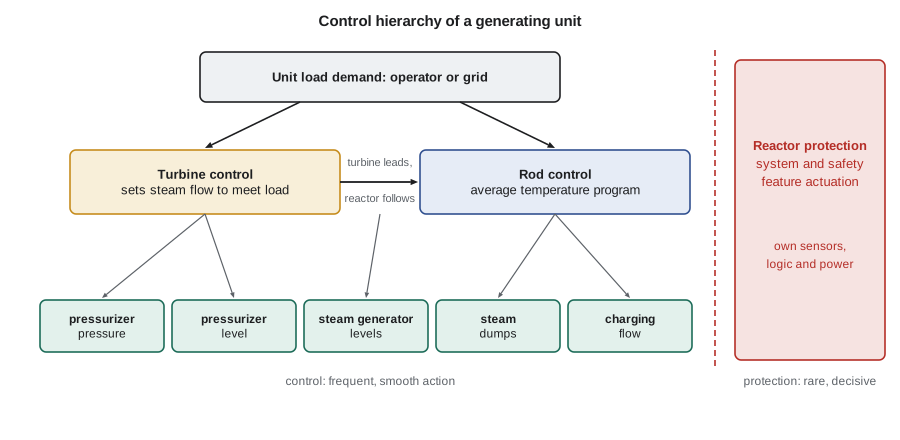
A nuclear generating unit is controlled at several levels. At the top is the unit load demand, set by the operator or by the grid dispatcher. In a typical pressurized water reactor the turbine leads and the reactor follows: the turbine control system sets steam flow to meet the load, and the reactor control system moves control rods to keep the average reactor coolant temperature on a program that rises with load. Below this level sit dozens of loops for pressurizer pressure and level, steam generator levels, steam dumps, feedwater pump speed and charging flow, each with its own controller. A boiling water reactor uses yet another arrangement: power is adjusted with recirculation flow and control rods, while the pressure regulator positions the turbine control valves to hold reactor pressure. The natural-circulation BWRX-300 has no recirculation pumps, so it adjusts power with fine-motion control rods and feedwater temperature.
Separating control from protection
The most important design principle in reactor instrumentation is that control and protection are separate. The control systems keep the plant at its desired operating point and are designed for good performance. The reactor protection system and the engineered safety features actuation system watch for conditions that the control systems failed to prevent and act to trip the reactor and start safety systems. If a control failure could also disable the protection that is meant to catch it, one fault could both cause an accident and prevent the response. IEEE 603, incorporated into 10 CFR 50.55a(h), and IEEE 279 before it, therefore require that where a signal is shared between control and protection, a single failure that causes a control action requiring protection cannot also prevent that protective action, and that protection channels be isolated from control circuits by qualified isolation devices.
Separation is also behavioral. Control systems are expected to act often and smoothly; protection systems are expected to act rarely and decisively. A control system that saturates or misbehaves is a nuisance; a protection system that fails to act is a potential accident. The two are therefore designed, qualified, maintained and changed under different rules, with protection held to the highest safety classification. Later lessons build on this distinction in detail.
Worked problem
Choosing a structure
A steam generator's level is disturbed mainly by changes in steam flow when the turbine load changes, and the feedwater valve's flow characteristic changes with feed pump discharge pressure. Which control structure addresses each problem?
Show solution
- The steam flow change is a measurable disturbance, so feedforward from steam flow lets feed flow change before the level moves.
- The valve and pump pressure changes act on feed flow, so an inner flow loop in cascade corrects them before they reach level.
- Level feedback trims the remaining error and handles anything not modeled.
Answer: Use feedforward from steam flow, a cascade inner loop on feed flow and outer feedback on level: the three-element controller.
Common mistakes
MistakeIntegral action makes a loop faster.
InsteadIntegral action removes offset but adds lag; too much of it causes overshoot.
MistakeA higher gain always gives tighter control.
InsteadBeyond a point higher gain causes oscillation, especially with dead time.
MistakeControl and protection can share a computer if the software is good.
InsteadProtection must be independent of control so that one failure cannot cause an event and disable the response.
Summary and key terms
- Feedback compares a measurement with a setpoint and acts on the error; feedforward acts on a measured disturbance.
- Proportional, integral and derivative actions trade speed, offset and noise sensitivity.
- Dead time and lags limit how tightly a loop can be tuned; gain and phase margins measure stability.
- Cascade and ratio structures split a problem into faster and slower parts.
- Protection systems are kept independent of control systems.
- Setpoint
- The desired value of a controlled variable.
- Error
- Setpoint minus measured value.
- Integral windup
- Accumulation of integral action while the output is saturated.
- Dead time
- A pure delay before a change reaches the measurement.
- Phase margin
- Extra phase lag a loop can tolerate at unity loop gain before it becomes unstable.
- Cascade control
- A structure in which one controller sets the setpoint of another.
Practice problems
Work each problem on paper first, then reveal the answer to check.
Why does proportional-only control leave an offset?
Show answer
Some error is needed to hold the controller output away from its resting value.
What is integral windup and how is it prevented?
Show answer
Integral accumulation while the output is at a limit; stop integrating when saturated.
Why is derivative action rarely used on flux or flow signals?
Show answer
Those signals are noisy, and derivative action amplifies noise.
State the condition for cascade control to work well.
Show answer
The inner loop must be several times faster than the outer loop.
Describe the usual PWR unit control mode.
Show answer
Turbine leading: the turbine meets load and rods keep average temperature on program.
Lesson quiz · 5 questions
Score 60% or more to complete this lesson.
Create a free account to save your progress, take quizzes and earn a certificate.