
MSAZ-320 · Lesson 7 of 12 · 21 min
Transforming data with T-SQL in the warehouse
▶ Video coming soon A video version of this lesson is on the way.
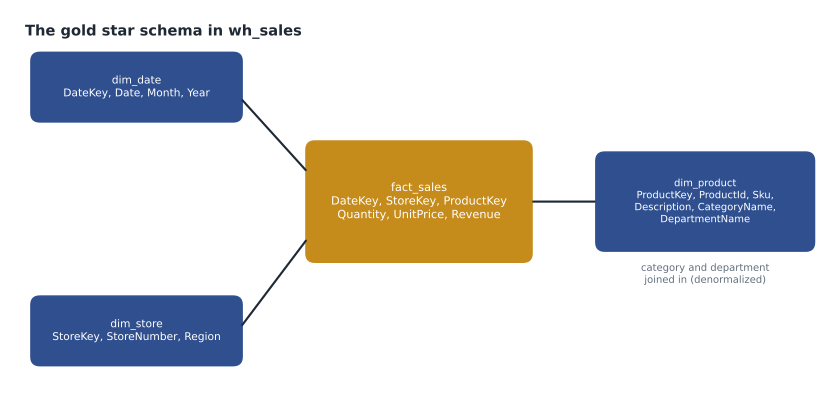
Tuesday, November 3, belonged to the gold layer. The curated tables in lh_curated were clean, but reports need a different shape: a fact table of sales lines with small integer keys pointing to dimension tables for date, store and product, the star schema that Power BI models read fastest and analysts understand at a glance. The hub's design put that star schema in the warehouse wh_sales, built with T-SQL, and Walt Hadley came to the afternoon session because he would be the one reviewing the procedures.
MSAZ-310 covered what a warehouse is: full T-SQL with inserts, updates, deletes and multi-table transactions, cross-database queries by three-part name, zero-copy clones and restore points. This lesson is about using those capabilities to load and transform data.
Getting data into the warehouse
The warehouse can read the lakehouse directly. A cross-database query names a lakehouse's SQL analytics endpoint table by its three-part name, such as lh_curated.stockline.sales, as long as both items are in the same workspace and the user can read both. That makes INSERT ... SELECT and CREATE TABLE AS SELECT, usually shortened to CTAS, the main loading tools: they read curated tables and write warehouse tables in one set-based statement, with no data leaving Fabric.
| Method | Reads from | Typical use |
|---|---|---|
| CTAS | Tables and views in the workspace's warehouses, lakehouse endpoints and mirrored databases; OPENROWSET over files | Create a new table from a query, such as a rebuilt dimension |
| INSERT ... SELECT | The same | Add rows to an existing table, such as a day of facts |
| COPY INTO | CSV, JSONL or Parquet files in Azure storage or OneLake | High-throughput bulk loads from files |
| OPENROWSET | Parquet, CSV or JSONL files in ADLS Gen2 or Blob storage | Read a file ad hoc in a query |
| Pipelines and dataflows | Many sources | Scheduled loads from outside Fabric |
COPY INTO is the fastest way to load files. It reads CSV, JSONL or Parquet files from an Azure storage account or a OneLake folder, and can sign in with the workspace identity, in which case the identity needs read access to the source and the person running the statement needs at least the Viewer role and INSERT on the target table. Without a credential, it uses the signed-in user's Microsoft Entra identity. Ines used it once, for the supplier price files, which arrive as CSV in the supplier storage account.
COPY INTO dbo.stg_supplier_price
FROM 'https://sthfsuppliercc.dfs.core.windows.net/prices/2026/11/*.csv'
WITH (
    FILE_TYPE  = 'CSV',
    FIRSTROW   = 2,
    CREDENTIAL = (IDENTITY = 'Workspace Identity')
);
On the US site the storage account is sthfsuppliercus; everything else is the same. Microsoft's guidance is to keep files at least about 4 megabytes and to split very large compressed CSV files, because COPY INTO reads many files in parallel.
Building dimensions
A dimension table describes something the business measures by: a store, a product, a date. Each row has a surrogate key, a small integer created by the warehouse, alongside the business key from the source, such as the StockLine ProductId. Surrogate keys keep the fact table narrow, survive changes in source systems and, as lesson 9 shows, allow one product to have several historical versions. A dimension is also where data is denormalized: product category and department, which StockLine keeps in separate tables, are joined into the product dimension so reports never have to join them again.
CREATE TABLE dbo.dim_product
AS
SELECT
    ROW_NUMBER() OVER (ORDER BY p.ProductId) AS ProductKey,       -- surrogate key
    p.ProductId,                                                   -- business key
    p.Sku, p.Description, c.CategoryName, d.DepartmentName,
    p.UnitPrice
FROM lh_curated.stockline.products    AS p
JOIN lh_curated.stockline.categories  AS c ON c.CategoryId   = p.CategoryId
JOIN lh_curated.stockline.departments AS d ON d.DepartmentId = c.DepartmentId;
Generating keys with ROW_NUMBER works for a first build. For later loads, new products need keys that continue from the largest existing key, which the stored procedure in the next section does. Check the current warehouse documentation for identity column support before relying on it; the ROW_NUMBER approach works everywhere and makes the rule visible in the code.
Loading facts in a transaction
The fact table holds one row per sale line: the date key, store key and product key, plus measures such as quantity, unit price and revenue. Loading it means looking up each line's keys in the dimensions. Because the warehouse supports multi-table transactions, the nightly procedure can add new products to dim_product and the day's sales to fact_sales together: if anything fails, both changes roll back and the gold layer stays consistent.
CREATE PROCEDURE dbo.load_day @LoadDate date
AS
BEGIN
    BEGIN TRANSACTION;

    -- 1. new products get keys after the current maximum
    DECLARE @MaxKey int = (SELECT COALESCE(MAX(ProductKey), 0) FROM dbo.dim_product);
    INSERT INTO dbo.dim_product (ProductKey, ProductId, Sku, Description, CategoryName, DepartmentName, UnitPrice)
    SELECT @MaxKey + ROW_NUMBER() OVER (ORDER BY p.ProductId), p.ProductId, p.Sku, p.Description,
           c.CategoryName, d.DepartmentName, p.UnitPrice
    FROM lh_curated.stockline.products p
    JOIN lh_curated.stockline.categories c  ON c.CategoryId = p.CategoryId
    JOIN lh_curated.stockline.departments d ON d.DepartmentId = c.DepartmentId
    WHERE NOT EXISTS (SELECT 1 FROM dbo.dim_product x WHERE x.ProductId = p.ProductId);

    -- 2. replace the day's facts, so a rerun cannot double-count
    DELETE FROM dbo.fact_sales WHERE DateKey = CONVERT(int, FORMAT(@LoadDate, 'yyyyMMdd'));
    INSERT INTO dbo.fact_sales (DateKey, StoreKey, ProductKey, Quantity, UnitPrice, Revenue)
    SELECT CONVERT(int, FORMAT(s.SaleDate, 'yyyyMMdd')), st.StoreKey, pr.ProductKey,
           s.Quantity, s.UnitPrice, s.Quantity * s.UnitPrice
    FROM lh_curated.stockline.sales s
    JOIN dbo.dim_store   st ON st.StoreNumber = s.StoreNumber
    JOIN dbo.dim_product pr ON pr.ProductId   = s.ProductId
    WHERE s.SaleDate = @LoadDate;

    COMMIT TRANSACTION;
END;
Walt's review comment was about step 2. Deleting the day's facts before inserting them makes the procedure idempotent: running it twice for the same date gives the same result as running it once. Without the delete, a pipeline retry after a timeout would have doubled a day's revenue. Idempotent loads are one of the habits DP-700 looks for, and lesson 8 returns to them.
The same pattern on a small scale
The SQL above cannot run in a browser, but the pattern can. Ines rebuilt it with Python's built-in SQLite database on five sales lines, so Keiko could watch the keys being assigned and the facts joined.
import sqlite3
db = sqlite3.connect(":memory:")
db.executescript("""
CREATE TABLE products (ProductId INT, Sku TEXT, Category TEXT);
INSERT INTO products VALUES (9001,'PNT-114','Paint'),(9002,'BRS-030','Paint'),(9003,'HMR-016','Tools');
CREATE TABLE sales (SaleDate TEXT, Store INT, ProductId INT, Qty INT, Price REAL);
INSERT INTO sales VALUES ('2026-11-02',12,9001,2,42.99),('2026-11-02',12,9002,3,6.49),
                         ('2026-11-02',15,9001,1,42.99),('2026-11-02',15,9003,1,24.99),
                         ('2026-11-02',15,9002,2,6.49);
CREATE TABLE dim_product AS
  SELECT ROW_NUMBER() OVER (ORDER BY ProductId) AS ProductKey, ProductId, Sku, Category FROM products;
CREATE TABLE fact_sales AS
  SELECT CAST(REPLACE(s.SaleDate,'-','') AS INT) AS DateKey, s.Store, d.ProductKey,
         s.Qty, ROUND(s.Qty * s.Price, 2) AS Revenue
  FROM sales s JOIN dim_product d ON d.ProductId = s.ProductId;
""")
print("dim_product:", db.execute("SELECT ProductKey, Sku FROM dim_product").fetchall())
for row in db.execute("SELECT d.Category, SUM(f.Revenue) FROM fact_sales f JOIN dim_product d USING (ProductKey) GROUP BY d.Category"):
print("revenue by category:", row[0], round(row[1], 2))dim_product: [(1, 'PNT-114'), (2, 'BRS-030'), (3, 'HMR-016')] revenue by category: Paint 161.42 revenue by category: Tools 24.99
What this code does
The program creates two small tables in memory, three products and five sale lines, then builds a product dimension that gives each product a new number, the surrogate key, in order of its product id. It builds a fact table by joining each sale line to that dimension so the line carries the short key instead of the product id, and it turns the sale date into a whole-number date key. Finally it joins facts back to the dimension and adds up revenue by category, which is exactly the kind of question a star schema is built to answer.
The output gives keys 1, 2 and 3 to the three products, and revenue of 161.42 for paint and 24.99 for tools. On the real data, the first build of dim_product created 61,412 rows and fact_sales 41.2 million, and Keiko's category report in Power BI returned in under two seconds.
Notebooks or T-SQL for the gold layer?
Spark could have built the star schema too, writing Delta tables in a lakehouse. The hub chose the warehouse for three reasons that DP-700 scenarios often turn on: the team that reviews the logic writes SQL; the load needs a multi-table transaction so that a failure never leaves new facts without their dimensions; and analysts wanted to create their own views and grant SQL permissions on the gold tables. A team of Python engineers with no SQL reviewers, loading tables that need no cross-table transaction, might reasonably choose a lakehouse gold layer instead.
Views, procedures and who may change what
The warehouse is also where the gold layer's rules about access are easiest to express. Analysts in sg-fdh-analysts can read the star schema through the SQL endpoint and the semantic model, but they cannot change the tables, because they hold the Viewer role and only SELECT permission. When an analyst needs a reusable calculation, such as revenue excluding returns, it becomes a view created by an engineer and reviewed in a pull request, so that every report uses the same definition. Stored procedures such as load_day are run by the pipeline under the workspace's identity, and nobody runs them by hand in production.
Keeping the transformation logic in procedures stored in Git, rather than in ad hoc scripts on someone's laptop, also gives the team a history. When finance asked in November why revenue for one day in 2025 differed from an old report, Walt could show the exact version of load_day that had produced it and the change, made in the rounding fix, that explained the difference.
Date dimensions
Every star schema needs a date dimension: one row per day, with columns for the day of the week, the month, the fiscal period, public holidays and anything else reports group or filter by. It is usually generated rather than loaded, with a short script that produces a row for every day across the range the business needs, often ten years back and two forward. Harrow & Finch's fiscal year starts on February 1, so dim_date carries both calendar and fiscal columns, and a column marking the days stores were closed, which the volume checks in lesson 12 use to avoid false alarms on public holidays.
Like the dimensions, dim_date has a surrogate key, but by convention it is a readable integer such as 20261102 rather than a counter, which is why the fact load converts each sale date into that form. Readable date keys make facts easy to check by eye and to filter by range, and because every day already exists in the dimension, no fact can ever arrive with a date the dimension lacks, a guarantee the store and product dimensions cannot offer and lesson 9 handles with inferred members.
Worked problem
Assign keys to new products
dim_product has 61,412 rows with keys 1 to 61,412. Tonight StockLine adds three products with ProductIds 77105, 77102 and 77110. Which keys will the procedure give them?
Show solution
- The procedure reads the current maximum key: 61,412.
- New products are numbered in ProductId order with ROW_NUMBER: 77102 first, 77105 second, 77110 third.
- Each key is the maximum plus its row number: 61,413, 61,414 and 61,415.
- Products already in the dimension are excluded by the NOT EXISTS condition, so rerunning the procedure adds no duplicates.
Answer: 77102 gets 61,413, 77105 gets 61,414 and 77110 gets 61,415.
Statistics, singleton inserts and performance
The warehouse creates and updates statistics automatically to plan queries. Two habits keep it fast. Load in sets with CTAS and INSERT ... SELECT, not with thousands of single-row INSERT statements, which perform poorly. And be aware that after a rolled-back transaction, automatically created statistics may describe rows that no longer exist, so updating statistics on the affected columns is good practice. MSAZ-321 covers warehouse performance in more depth.
Common mistakes
MistakeCopy curated tables into the warehouse with a pipeline before transforming them.
InsteadRead lakehouse endpoint tables directly with three-part names in CTAS or INSERT ... SELECT.
MistakeInsert the day's facts without removing earlier attempts.
InsteadDelete the day's facts first, or MERGE, so reruns are idempotent.
MistakeUse the source system's ProductId as the fact table's key.
InsteadUse a surrogate key from the dimension; keep the business key in the dimension.
MistakeLoad rows one INSERT at a time.
InsteadUse set-based CTAS or INSERT ... SELECT.
Summary and key terms
- The warehouse reads lakehouse endpoints and mirrored databases in the same workspace by three-part name.
- CTAS and INSERT ... SELECT are the main set-based loading tools; COPY INTO bulk-loads files.
- Dimensions carry surrogate keys, business keys and denormalized attributes.
- Multi-table transactions keep dimensions and facts consistent if a load fails.
- Deleting and reinserting a day's facts makes the load idempotent.
- Choose T-SQL when SQL people own the logic or cross-table transactions are needed.
- Star schema
- A design with a central fact table joined to dimension tables by keys.
- Fact table
- A table of measurable events, such as sale lines, with keys to dimensions.
- Dimension table
- A table describing an entity, such as a product or store, used to filter and group facts.
- Surrogate key
- A key created by the warehouse for a dimension row, independent of the source system.
- Business key
- The identifier used in the source system, such as ProductId.
- CTAS
- CREATE TABLE AS SELECT: creating a table from the result of a query.
- Idempotent load
- A load that gives the same result whether it runs once or several times.
Practice problems
Work each problem on paper first, then reveal the answer to check.
How does the warehouse read lh_curated.stockline.sales without copying it first?
Show answer
With a cross-database query using the three-part name.
Which file types can COPY INTO read?
Show answer
CSV, JSONL and Parquet.
Why does the procedure delete the day's facts before inserting them?
Show answer
So a rerun does not double-count; the load is idempotent.
What does a surrogate key protect against?
Show answer
Changes in source system keys, and it allows several versions of a row.
Name one reason the hub built its gold layer in a warehouse.
Show answer
For example SQL reviewers, multi-table transactions, or analysts managing SQL views and permissions.
Lesson quiz · 5 questions
Score 60% or more to complete this lesson.
Create a free account to save your progress, take quizzes and earn a certificate.