Production, costs and economies of scale and scope

Demand tells a manager what customers will pay; costs tell her what it takes to serve them. MBA-501 looked at costs through the lens of the accountant: fixed and variable, direct and indirect, product and period. This lesson looks at the same costs through the lens of the economist, who asks how costs change with the scale of output, with the length of the time horizon, with the range of products produced and with accumulated experience. These questions determine how large a plant should be, whether a merger can reduce costs, whether a firm should add a product line and how industries are likely to be structured.

Production and the short run

A production function describes the maximum output a firm can produce from given quantities of inputs such as labor, capital, materials and energy. In the short run, at least one input, typically capital such as a plant or a fleet of presses, is fixed. Adding more of a variable input, such as labor or shifts, to a fixed amount of capital eventually yields smaller and smaller additions to output. This is the law of diminishing marginal returns, and it is the reason short-run marginal cost curves eventually slope upwards.

Daniel Osei sees diminishing returns every quarter at Northfield. With two shifts on its six stamping presses, output per press-hour is high. Adding a third shift raises output, but less than proportionally: setup and maintenance time has to be squeezed into fewer windows, the newest operators work the night shift, scrap rates rise and supervisors are stretched. Overtime on weekends raises output again, but each extra hour costs a wage premium and yields still less. The marginal cost of a part therefore rises sharply as Northfield approaches the physical capacity of the presses.

Short-run cost curves

Short-run total cost is the sum of fixed cost, which does not change with output in the short run, and variable cost, which does. Dividing by output gives average fixed cost, which falls continuously as fixed costs are spread over more units, average variable cost, and average total cost. Marginal cost is the change in total cost from one more unit. Because of diminishing returns, marginal cost first falls and then rises, and it cuts both average variable cost and average total cost at their minimum points. The intuition is the same as for grade averages: if your next exam score is below your average, the average falls; if it is above, the average rises.

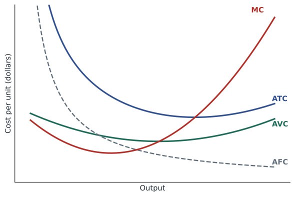
The distinction between average and marginal cost matters greatly in practice. A hospital with empty beds has a high average cost per patient-day, because fixed costs are spread over few patients, but a low marginal cost of admitting one more patient. A factory running near capacity may have a moderate average cost but a very high marginal cost of one more unit, because that unit requires overtime and expediting. Pricing and output decisions should be based on marginal cost; decisions about whether to stay in business should be based on whether price covers average cost in the long run.

The long run and economies of scale

In the long run all inputs can be varied: a firm can build a larger plant, buy more presses or open more stores. The long-run average cost curve shows the lowest average cost of producing each level of output when the firm can choose the best plant for that level. Economies of scale exist when long-run average cost falls as output rises; diseconomies of scale exist when it rises. Between them there is often a wide range of output with roughly constant average cost.

Economies of scale have many sources. Specialization of labor and equipment raises productivity in larger operations. Some costs are indivisible: a hospital needs one magnetic resonance imaging scanner whether it performs ten or thirty scans a day, and a software company spends almost the same to develop a product for a thousand or a million users. Engineering relationships give scale advantages in pipes, tanks, ships and gas plants, where capacity rises with volume while cost rises with surface area; the engineers' rule of thumb that the cost of process equipment rises roughly with capacity raised to the power 0.6 reflects this. Larger firms often pay less for inputs, borrow more cheaply and spread advertising and research over more sales.

Diseconomies of scale arise mainly from the difficulties of managing very large organizations: layers of hierarchy slow decisions, information is distorted as it travels, incentives weaken and coordination costs rise. Transport costs can also create diseconomies, because a single large plant must ship output farther than several smaller ones. Hana Kowalski at Lakeview Health sees both sides: consolidating laboratory testing into one central laboratory cut the cost per test, but consolidating all administrative decisions into a central office slowed decisions in the clinics and raised overtime costs.

Minimum efficient scale and industry structure

The minimum efficient scale is the smallest output at which long-run average cost reaches its minimum. Comparing it with the size of the market says a great deal about how many firms an industry can support. If minimum efficient scale is small relative to market demand, as in restaurants, hair salons and many professional services, the market can support many firms, and competition is likely to be intense. If it is large, as in aircraft manufacturing, oil refining, wireless networks and large-scale cloud computing, only a few firms can operate at efficient scale, and the industry tends to be concentrated. Lesson 6 explores the strategic behavior that results.

# Estimating economies of scale: processing cost at gas-processing plants of different sizes
# Owen's data on Prairie Ridge and four peer plants (capacity in thousand gigajoules per day, annual cost in millions)
import math
capacity = [60, 110, 180, 260, 400]
annual_cost = [21.5, 31.8, 43.9, 55.2, 72.6]
x = [math.log(c) for c in capacity]; y = [math.log(c) for c in annual_cost]
n = len(x); mx, my = sum(x) / n, sum(y) / n
b = sum((xi - mx) * (yi - my) for xi, yi in zip(x, y)) / sum((xi - mx) ** 2 for xi in x)
a = my - b * mx
print(f"Cost elasticity with respect to capacity: {b:.2f}  (below 1 means economies of scale)")
for c, tc in zip(capacity, annual_cost):
    print(f"  {c:3d} thousand GJ/day: average cost {tc / (c * 365) * 1e6:5.3f} dollars per GJ")
# cost of doubling a 180 plant using the estimated exponent
print(f"Predicted cost of a 360 plant: {math.exp(a + b * math.log(360)):.1f} million (vs {2 * 43.9:.1f} for two 180 plants)")

Cost elasticity with respect to capacity: 0.64  (below 1 means economies of scale)
   60 thousand GJ/day: average cost 981.735 dollars per GJ
  110 thousand GJ/day: average cost 792.030 dollars per GJ
  180 thousand GJ/day: average cost 668.189 dollars per GJ
  260 thousand GJ/day: average cost 581.665 dollars per GJ
  400 thousand GJ/day: average cost 497.260 dollars per GJ
Predicted cost of a 360 plant: 68.1 million (vs 87.8 for two 180 plants)

The estimated cost elasticity of about 0.6 means that a 10 % increase in plant capacity raises annual cost by only about 6 %, so average cost per gigajoule falls as plants get larger. Owen uses the estimate when Prairie Ridge considers whether to expand its main plant or build a second, smaller one closer to new wells: the larger plant has lower processing cost per gigajoule, but the smaller one saves pipeline costs and spreads the risk of an outage.

Economies of scope

Economies of scope exist when producing two or more products together costs less than producing them separately. They arise from shared inputs: a distribution network that carries many products, a brand that can be stretched across categories, research that benefits several product lines, or a customer relationship that supports several services. Fairway's stores achieve economies of scope by selling groceries, pharmacy items and prepared meals through the same buildings, staff and loyalty program. Prairie Ridge uses the same control room and field crews for its gas plant and its wind farms. A useful measure compares the cost of producing products jointly with the sum of the costs of producing them separately.

A positive value of S indicates economies of scope. Many mergers and diversifications are justified by claimed economies of scope, and many fail to deliver them, because shared resources become congested, complexity rises and the products turn out to need different capabilities. MBA-514 Business Strategy returns to the strategic question of when diversification creates value.

Learning curves

In many activities, unit cost falls as cumulative output grows, because workers become more skilled, engineers refine designs and processes, and suppliers improve. This learning, or experience, curve was documented in aircraft assembly in the 1930s and later popularized by the Boston Consulting Group. A common description is that unit cost falls by a constant percentage each time cumulative output doubles: an 80 % learning curve means the cost of the unit produced after cumulative output doubles is 80 % of the earlier unit. Solar panels and lithium-ion batteries have shown strong learning effects over several decades, which is one reason their prices have fallen so far.

Learning economies differ from economies of scale. Scale economies depend on the rate of output per period; learning depends on cumulative output over time. A small firm that has produced a product for many years can have lower costs than a larger newcomer, and a firm that cuts prices to build volume early can move down the learning curve faster than its rivals, a strategy whose risks Lesson 8 examines.

Costs that matter for decisions

Economic costs are opportunity costs, and the costs that matter for a decision are the ones that change with it. In the short run, fixed costs do not affect the output decision, but they do affect the decision to stay in business in the long run. Sunk costs never matter. Committed costs, such as a long-term lease, may be avoidable only at a penalty, which becomes the relevant cost of exit. Capacity costs matter for pricing when capacity is scarce: when Northfield's presses are full, the true marginal cost of an extra order includes the contribution from the work it displaces. This is the same logic as the constrained-resource decisions in MBA-501, seen from the economist's side.