Demand, elasticity and estimating demand from data

Revenue is price times quantity, and quantity depends on price. Every pricing, promotion and capacity decision therefore rests on some belief about demand: how many customers will buy at each price, and how sensitive they are to changes in price, income and the prices of related goods. This lesson develops the demand curve, the elasticities that summarize it, and the practical methods that managers use to estimate demand from data, from simple before-and-after comparisons to regression on sales records and experiments.

The demand curve and what shifts it

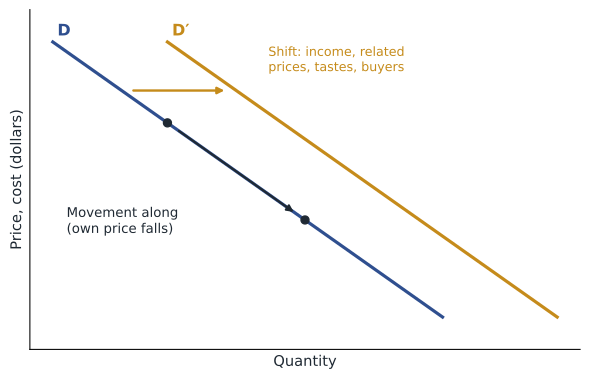
A demand curve shows the quantity buyers are willing and able to purchase at each price, holding everything else constant. It slopes downwards for almost all goods, for two reasons. When a good becomes cheaper, some buyers switch to it from substitutes, and buyers who already use it can afford a little more of everything, including the good itself. A movement along the demand curve is caused only by a change in the good's own price. Everything else that affects purchases shifts the whole curve: buyers' incomes, the prices of substitutes and complements, tastes and expectations, the number of buyers, advertising, and seasonal or weather effects.

Grace Mwangi manages the coffee category at Fairway Grocers, and the distinction between moving along and shifting the curve is the first thing she checks when sales change. A drop in coffee sales after Fairway raised its private-label price is a movement along the curve. A drop after a new discount chain opened nearby is a shift, because a substitute became more attractive at every price. A jump in sales of premium beans before a long weekend is a seasonal shift. Treating a shift as a movement, or the reverse, leads to wrong conclusions about how customers respond to price.

Price elasticity of demand

The slope of a demand curve depends on the units used, so economists summarize price sensitivity with the price elasticity of demand: the percentage change in quantity demanded divided by the percentage change in price. Because quantity falls when price rises, the elasticity is negative, and managers often quote its absolute value. Demand is elastic when the absolute value exceeds 1, so that quantity changes by a larger percentage than price, and inelastic when it is below 1.

For changes between two observed points, the midpoint or arc formula divides each change by the average of the two values, so that the answer is the same whether the price rises or falls. For small changes, or when demand has been estimated as an equation, the point elasticity uses the slope of the curve at a particular point.

Elasticity matters because it tells a manager what happens to revenue when price changes. If demand is inelastic, a price increase loses relatively few sales and total revenue rises. If demand is elastic, a price increase loses so many sales that total revenue falls. At unit elasticity revenue does not change. For profit, rather than revenue, the cost side also matters, and Lesson 3 shows that a profit-maximizing firm always sets price where demand is elastic. A manager who discovers that demand at the current price is inelastic has, in effect, discovered that the price is too low.

What makes demand elastic or inelastic

Demand tends to be more elastic when close substitutes are available, when the good takes a large share of the buyer's budget, when buyers have time to adjust and when the market is defined narrowly. Demand for a particular brand of coffee at a particular store is far more elastic than demand for coffee in general, because shoppers can switch brands or stores. Demand for gasoline is inelastic in the short run, because people cannot quickly change cars or commutes, but considerably more elastic over several years. Demand for insulin is very inelastic for the individual patient, which is one reason that drug prices attract regulation.

Empirical studies give a sense of magnitudes, although estimates vary widely by market and method. Short-run gasoline demand elasticities are commonly estimated between about −0.1 and −0.3, with long-run estimates several times larger. Elasticities for individual grocery brands are often in the range of −2 to −4, while those for broad food categories are well below 1 in absolute value. Elasticities for air travel are higher for leisure travelers than for business travelers, which explains much of airline pricing. These are illustrative ranges rather than rules; every business should estimate its own.

Income and cross-price elasticities

The income elasticity of demand measures how quantity responds to income. Normal goods have positive income elasticity; luxuries have an income elasticity above 1, so their share of spending rises as people become richer; inferior goods have negative income elasticity, so demand falls as incomes rise. Private-label groceries behave partly as inferior goods: Fairway's private-label share rose during the inflation of 2022 and 2023, when household budgets were squeezed, and fell back slightly as real incomes recovered. Owen Tremblay sees the same idea at Prairie Ridge Energy: industrial gas demand moves with economic activity, while residential heating demand barely responds to income at all.

The cross-price elasticity measures how the quantity of one good responds to the price of another. A positive cross elasticity means the goods are substitutes, such as two brands of coffee or natural gas and electricity for heating. A negative cross elasticity means they are complements, such as printers and ink cartridges, or the coffee and the cream that shoppers buy with it. Retailers use cross elasticities to design promotions: a loss-leader works only if the discounted item is a complement to other items with healthy margins. Competition authorities use them to define markets, because goods with high cross elasticities compete with one another.

Estimating demand from data

Managers can learn about demand in several ways. Surveys and conjoint analysis ask customers to choose between hypothetical products and prices; they are cheap and flexible but tell you what people say rather than what they do. Historical sales data show what people actually did, but prices in the data rarely changed for random reasons, which creates a serious problem discussed below. Experiments, including the online A/B tests that software companies run constantly and the price tests that retailers run in matched stores, provide the cleanest evidence because the manager controls the variation in price.

The workhorse statistical method is regression. A common specification is the constant-elasticity or log-log demand curve, in which the logarithm of quantity is a linear function of the logarithm of price and other variables. The coefficient on log price is then the price elasticity, and the coefficients on log income or log competitor price are the income and cross elasticities. The specification is popular because it is simple, it fits many markets reasonably well and its coefficients have a direct interpretation.

# Estimating the price elasticity of Fairway's private-label coffee from 12 weeks of store data
import math
price = [11.49, 11.49, 10.99, 11.99, 12.49, 10.49, 11.49, 12.99, 10.99, 11.99, 9.99, 12.49]   # dollars per bag
bags  = [ 940,   905,  1035,   830,   745,  1150,   920,   690,  1010,   850,  1290,   760]
x = [math.log(p) for p in price]; y = [math.log(q) for q in bags]
n = len(x); mx, my = sum(x) / n, sum(y) / n
b = sum((xi - mx) * (yi - my) for xi, yi in zip(x, y)) / sum((xi - mx) ** 2 for xi in x)
a = my - b * mx
resid = [yi - (a + b * xi) for xi, yi in zip(x, y)]
r2 = 1 - sum(e * e for e in resid) / sum((yi - my) ** 2 for yi in y)
print(f"Estimated price elasticity {b:.2f}  (R-squared {r2:.2f})")
# arc elasticity between two observed weeks
p1, q1, p2, q2 = 10.99, 1035, 11.99, 830
arc = ((q2 - q1) / ((q1 + q2) / 2)) / ((p2 - p1) / ((p1 + p2) / 2))
print(f"Arc elasticity between 10.99 and 11.99: {arc:.2f}")
for change in (-0.05, 0.05):
    q_new = math.exp(a + b * math.log(11.49 * (1 + change)))
    print(f"Price {change:+.0%}: predicted bags {q_new:5.0f}, revenue {11.49 * (1 + change) * q_new:8.0f} dollars")

Estimated price elasticity -2.39  (R-squared 1.00)
Arc elasticity between 10.99 and 11.99: -2.53
Price -5%: predicted bags  1043, revenue    11385 dollars
Price +5%: predicted bags   821, revenue     9909 dollars

The estimated elasticity of about −2.7 says that a 1 % price increase reduces bags sold by roughly 2.7 %, so demand for this brand at this store is elastic and a price cut increases revenue. Whether it increases profit depends on the margin, which Lesson 3 takes up. Grace knows that twelve weeks is a short sample and that the estimate has a wide confidence interval, so she treats it as a starting point for a controlled test rather than as a final answer.

The identification problem

Historical prices are usually set by managers who respond to demand. If Fairway raised prices when it expected strong demand, for example before holidays, and cut prices when demand was weak, the data will show high prices paired with high sales, and a naive regression may suggest that demand curves slope upwards. More generally, observed prices and quantities are the result of both supply and demand shifting, and separating the two requires variation in price that is not caused by demand shocks. Economists call this the identification problem.

Several solutions are available. Experiments create price variation that is unrelated to demand by design. Instrumental variables use factors that shift costs or supply but not demand, such as a change in a commodity input price, to isolate movements along the demand curve. Controlling for the known demand shifters, such as seasons, holidays, weather and competitor promotions, reduces the bias. And natural experiments, such as a tax change in one province or state but not its neighbor, can provide credible evidence. Leo's team at Kestrel now runs randomized price tests on new sign-ups, a common practice among subscription software companies, because it removes the identification problem almost entirely.

Using elasticities in decisions

Elasticities feed directly into decisions. A retailer can calculate how much a promotion must lift volume to pay for itself. A utility can forecast how a rate increase will affect consumption and revenue. A manufacturer can estimate how much of a cost increase it can pass on to customers. Daniel Osei at Northfield uses a simple version for contract negotiations: because the auto makers he supplies have alternative suppliers for most stampings, the effective elasticity of demand facing Northfield for a standard bracket is high, so he expects to absorb most of a steel price increase. For a complex welded assembly with few qualified suppliers, demand is much less elastic and he can pass more of the increase through.

Elasticities also change over time and with market conditions. They are larger in the long run, as buyers find substitutes; they rise when competitors cut prices and fall when competitors leave; and they differ among customer segments. The single most common mistake is to treat an elasticity estimated in one setting as a constant that applies everywhere. Good practice is to estimate elasticities by segment and season, to update them regularly, and to test them before acting on large price changes.