Product and service costing: job, process and activity-based costing

What does it cost to make one bracket, treat one patient or serve one customer? The answer drives pricing, product decisions, inventory valuation and the profitability reports managers act on. Yet the cost of a product is not a fact waiting to be measured; it is the result of choices about which costs to include and how to assign shared costs. This lesson explains the two classic costing systems, job costing and process costing, shows how overhead is allocated, and explains why activity-based costing often reveals that some products and customers are far less profitable than they appear.

Direct and indirect costs

A direct cost can be traced to a cost object, such as a product, job, customer or department, in an economically feasible way. Steel in a Northfield bracket and the surgeon's time in a Lakeview procedure are direct. An indirect cost, or overhead, is shared by many cost objects and cannot be traced to any one of them economically: the plant manager's salary, building depreciation, quality inspection, information systems. Manufacturing cost traditionally has three parts, direct materials, direct labor and manufacturing overhead. Inventory and cost of goods sold in the financial statements include all three, a method called absorption or full costing.

In many modern businesses overhead is the largest category. At Northfield, direct materials are about 55 % of manufacturing cost and direct labor about 12 %, so overhead is a third. At Kestrel, almost all costs are indirect with respect to any one customer. When overhead is large, how it is assigned matters enormously.

Job costing

Job costing accumulates costs for each distinct job, batch or contract. It suits businesses that produce customized products or services: Northfield's tooling projects, a construction company's buildings, a consulting firm's engagements, a hospital's individual surgeries. Each job has a cost record showing the direct materials issued to it, the direct labor hours charged to it, and overhead applied using a predetermined rate.

The predetermined overhead rate is estimated at the start of the year by dividing budgeted overhead by a budgeted allocation base, such as direct labor hours or machine hours. During the year, overhead is applied to each job by multiplying its actual use of the base by the rate. Because the rate is an estimate, applied overhead rarely equals actual overhead exactly; the difference, under- or over-applied overhead, is usually closed to cost of goods sold at year-end or prorated across inventory and cost of goods sold.

# Job costing with a predetermined overhead rate (dollars)
budget_overhead, budget_machine_hours = 6_840_000, 72_000
rate = budget_overhead / budget_machine_hours
job = {"materials": 48_600, "direct work hours": 410, "wage rate": 38.50, "machine hours": 260}
direct_work = job["direct work hours"] * job["wage rate"]
applied = job["machine hours"] * rate
total = job["materials"] + direct_work + applied
print(f"Overhead rate {rate:.2f} dollars per machine hour")
print(f"Job T-4471: materials {job['materials']:,}  direct work {direct_work:,.0f}  overhead {applied:,.0f}  total {total:,.0f}")
actual_overhead, actual_machine_hours = 6_910_000, 70_400
applied_year = actual_machine_hours * rate
print(f"Year end: applied {applied_year:,.0f}, actual {actual_overhead:,.0f}, under-applied {actual_overhead - applied_year:,.0f}")

Overhead rate 95.00 dollars per machine hour
Job T-4471: materials 48,600  direct work 15,785  overhead 24,700  total 89,085
Year end: applied 6,688,000, actual 6,910,000, under-applied 222,000

Northfield quoted the T-4471 die set to its customer at cost plus 25 %. Daniel noticed that the overhead rate assumed the plant would run 72,000 machine hours, but a slow first half meant only about 70,000. With lower volume, actual overhead per hour was higher than the predetermined rate, so the company had under-applied overhead of about 222,000 dollars, a reminder that cost-plus quotes depend on volume assumptions.

Process costing

Process costing suits businesses that produce large volumes of identical units in a continuous flow: refining, food processing, chemicals, paper, and Northfield's high-volume stamping lines. Instead of tracing costs to individual jobs, it accumulates costs by process or department for a period and divides by the units produced. The complication is work in process at the start and end of the period: partly finished units are converted into equivalent units, the number of complete units their work represents. A batch of 10,000 brackets half-way through welding counts as 5,000 equivalent units of welding cost.

Process costing produces an average cost per unit, which is appropriate when units really are alike. Many businesses use hybrids: Fairway's bakery uses process costing for its standard loaves and job costing for custom cakes, and Northfield's operation costing tracks materials by job and conversion costs by process.

Service costing

Service organizations face the same questions with different words. Lakeview Health needs the cost of a clinic visit, an MRI scan or a hip replacement to negotiate with insurers and government funders and to decide which services to expand. Its costs are dominated by staff time, equipment and facilities shared across many patients. Time-driven costing works well in such settings: estimate the cost per minute of each resource, such as nurses, operating rooms or imaging equipment, and the minutes each service uses, then add them up. Hana's team found that a simple procedure performed in the main hospital cost 40 % more than the same procedure in an outpatient clinic, mainly because hospital operating room minutes carry the cost of capacity reserved for emergencies.

The problem with a single overhead rate

Traditional costing systems often allocate all overhead using one volume-based driver, such as direct labor hours or machine hours. That works when overhead really varies with volume. But much overhead is driven by complexity: the number of setups, purchase orders, engineering changes, inspections, customer orders and product variants. A low-volume, complex product causes far more of these activities per unit than a high-volume standard product, yet a volume-based rate charges both the same per hour. The result is systematic cross-subsidy: high-volume standard products are over-costed and low-volume specialty products are under-costed.

The distortion is not merely academic. A company that prices on cost will overprice its standard products, losing them to focused competitors, and underprice its specialty products, winning business that loses money. Over time the product line drifts toward complexity and margins fall, even though every product appears profitable on the reports.

Activity-based costing

Activity-based costing (ABC), developed in the 1980s by Robin Cooper and Robert Kaplan among others, assigns overhead in two stages. First, overhead is traced to activities, such as setting up machines, handling materials, inspecting, processing customer orders and supporting engineering changes. Second, the cost of each activity is assigned to products, services or customers using an activity driver that reflects how much of the activity each one consumes: number of setups, number of moves, inspection hours, number of orders. Because the drivers capture complexity, ABC assigns more cost to products and customers that demand more activity.

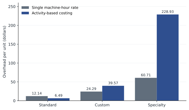
# Traditional versus activity-based costing for three Northfield products (overhead only, dollars)
products = {
    #           units    machine hrs  setups  inspections  engineering changes
    "Standard":  (400_000, 40_000,     40,     120,         4),
    "Custom":    (60_000,  12_000,     180,    420,         36),
    "Specialty": (8_000,   4_000,      140,    300,         60),
}
pools = {"machine hrs": 3_100_000, "setups": 1_440_000, "inspections": 1_260_000, "engineering changes": 1_000_000}
total_overhead = sum(pools.values())
total_mh = sum(p[1] for p in products.values())
idx = {"machine hrs": 1, "setups": 2, "inspections": 3, "engineering changes": 4}
driver_totals = {k: sum(p[i] for p in products.values()) for k, i in idx.items()}
for name, p in products.items():
    trad = total_overhead * p[1] / total_mh / p[0]
    abc = sum(pools[k] * p[i] / driver_totals[k] for k, i in idx.items()) / p[0]
    print(f"{name:<10} overhead per unit: traditional {trad:7.2f}   activity-based {abc:7.2f}")

Standard   overhead per unit: traditional   12.14   activity-based    6.49
Custom     overhead per unit: traditional   24.29   activity-based   39.57
Specialty  overhead per unit: traditional   60.71   activity-based  228.93

Under a single volume-based rate, the specialty product carries about 61 dollars of overhead per unit, but under ABC its overhead rises to about 229 dollars, nearly four times as much, because it uses a large share of the setups, inspections and engineering changes for a small number of units. The custom product rises from about 24 to about 40 dollars, while the standard product's overhead per unit roughly halves, from about 12 to about 6.50 dollars. Daniel's reaction was the typical one: "So the products sales loves are the ones losing money." The ABC results do not by themselves say to drop the specialty product. They say to price it properly, reduce the activities it consumes, or decide that it is strategically worth subsidizing.

Customer profitability

The same logic applies to customers. Two customers buying the same products can cost very different amounts to serve: one orders monthly in full truckloads with standard packaging and pays on time; another orders weekly in small lots, demands expedited shipping and special labeling, returns goods and pays late. Customer profitability analysis assigns order-handling, delivery, support and credit costs to customers. It often produces a whale curve: a minority of customers generates more than all of the profit, the middle group roughly breaks even, and a tail of customers destroys a large share of the profit the best customers create.

Kestrel ran this analysis and found that its smallest customers, on the cheapest plan, consumed a disproportionate share of support tickets and onboarding time. The response was not to drop them but to move them to self-service onboarding and a support community, which cut the cost to serve while keeping the customers, many of whom would grow into larger accounts.

Costs of implementing ABC

ABC is not free. Interviewing staff, mapping activities, collecting driver data and maintaining the model take time, and early ABC systems often collapsed under their own complexity. Time-driven ABC simplifies the approach by estimating the cost per minute of capacity and the minutes each transaction takes, which also reveals unused capacity, the cost of resources that are paid for but not used. Most companies do not need ABC for every decision; they use it periodically to check the product and customer profitability that their regular systems report.

Time-driven activity-based costing

The classic version of ABC requires interviewing staff about how they spend their time and updating those surveys as activities change, which is one reason many early systems were abandoned. Time-driven ABC, proposed by Robert Kaplan and Steven Anderson, simplifies the approach. It needs only two estimates for each department: the cost per minute of the capacity supplied, and the number of minutes each activity takes. The cost of processing an order, for example, is the minutes required multiplied by the cost per minute, and the minutes can vary with the order's characteristics, such as the number of lines or whether it is shipped overseas.

Time-driven ABC has a further advantage: it reveals unused capacity. If a department supplies 40,000 minutes a month and the activities measured consume 32,000, the cost of the remaining 8,000 minutes is shown separately as idle capacity rather than being spread over products. Managers can then decide whether to redeploy those resources, reduce them, or use them for growth. Leo Brandt adapted the approach at Kestrel Analytics to measure the cost of customer onboarding and support, and found that a handful of customers with custom data integrations consumed almost half of the support team's time.