Cost behavior and cost-volume-profit analysis

The second half of this course turns from reporting to deciding. Most managerial decisions start with a simple question: if we do more, or less, of something, what happens to cost and profit? Answering it requires understanding how costs behave as activity changes. This lesson classifies costs by behavior, shows how to estimate cost behavior from data, and develops cost-volume-profit (CVP) analysis, the most widely used model in managerial accounting, together with break-even, margin of safety and operating leverage.

Fixed, variable and mixed costs

A variable cost changes in total in proportion to activity: steel for each bracket Northfield stamps, the cost of each grocery item Fairway sells, payment-processing fees for each Kestrel subscription. Per unit it is constant. A fixed cost stays the same in total over a relevant range of activity: rent, salaried supervision, insurance, depreciation on a press. Per unit it falls as volume rises. A mixed, or semi-variable, cost has both parts, such as a utility bill with a fixed monthly charge plus a charge per kilowatt-hour, or a maintenance budget with routine and usage-driven elements. A step cost is fixed over a range and then jumps, such as adding a supervisor for every additional shift.

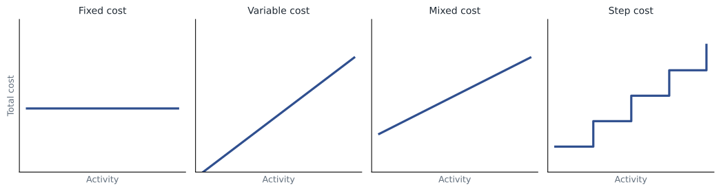
The relevant range matters. Northfield's plant costs are fixed for volumes up to the capacity of two shifts, but beyond that the company must add a third shift, overtime premiums or another press. Over a very long period nearly all costs become variable, because a company can sell a plant or close a store. Classifying costs is therefore always a statement about a particular range of activity and time horizon.

Activity can be measured in many ways: units produced, machine hours, patient visits, transactions, customers served, kilometers driven. The right measure, the cost driver, is the one that actually causes the cost to change. Lakeview's laboratory costs are driven by the number of tests, not the number of patients; Kestrel's cloud hosting costs are driven by the volume of data processed, not the number of customers. Lesson 9 shows that choosing better cost drivers changes product costs.

Estimating cost behavior

Managers rarely receive cost behavior ready-made. They estimate it from records. Account analysis classifies each ledger account as fixed, variable or mixed using judgment. The engineering method builds up cost from standards, such as kilograms of steel and minutes of machine time per part. Statistical methods use historical data on total cost and activity. The simplest is the high-low method, which draws a line through the periods with the highest and lowest activity; more reliable is least-squares regression, which fits the line that minimizes squared errors across all periods.

# Estimating fixed and variable maintenance cost at Northfield from 12 months of data
machine_hours = [3100, 3420, 2880, 3650, 3980, 3300, 2750, 3550, 4120, 3870, 3210, 2960]
cost = [148.0, 156.5, 141.2, 162.0, 171.4, 152.2, 139.0, 158.9, 176.3, 168.1, 150.6, 145.5]   # thousands
# high-low method
hi, lo = machine_hours.index(max(machine_hours)), machine_hours.index(min(machine_hours))
b_hl = (cost[hi] - cost[lo]) / (machine_hours[hi] - machine_hours[lo])
a_hl = cost[hi] - b_hl * machine_hours[hi]
# least-squares regression
n = len(cost)
mx, my = sum(machine_hours) / n, sum(cost) / n
sxy = sum((x - mx) * (y - my) for x, y in zip(machine_hours, cost))
sxx = sum((x - mx) ** 2 for x in machine_hours)
b = sxy / sxx
a = my - b * mx
ss_res = sum((y - (a + b * x)) ** 2 for x, y in zip(machine_hours, cost))
ss_tot = sum((y - my) ** 2 for y in cost)
print(f"High-low:   fixed {a_hl:6.1f} thousand per month, variable {1000 * b_hl:5.2f} dollars per machine hour")
print(f"Regression: fixed {a:6.1f} thousand per month, variable {1000 * b:5.2f} dollars per machine hour, R-squared {1 - ss_res / ss_tot:.3f}")
print(f"Predicted cost at 3,800 hours: {a + b * 3800:6.1f} thousand")

High-low:   fixed   64.1 thousand per month, variable 27.23 dollars per machine hour
Regression: fixed   65.0 thousand per month, variable 26.72 dollars per machine hour, R-squared 0.996
Predicted cost at 3,800 hours:  166.5 thousand

The two methods give similar answers here because the data are well behaved, but the high-low method uses only two points, and if either is unusual, perhaps a month with a major breakdown, the estimate can be badly wrong. Regression uses all the data and reports how well the line fits. Even a good fit describes the past; a new maintenance contract or aging equipment can change the relationship. Correlation is also not causation: a cost that rises with machine hours might really be driven by the number of setups, which happens to move with hours.

Contribution margin

The key concept in CVP analysis is the contribution margin: revenue minus variable costs. Per unit, it is the selling price minus the variable cost per unit, and it measures how much each unit contributes toward covering fixed costs and then to profit. The contribution margin ratio divides contribution by revenue. A contribution format income statement, which separates variable and fixed costs instead of grouping costs by function, makes these numbers visible, which is why managers use it internally even though external reports are prepared on a functional basis.

Here P is price per unit, V variable cost per unit, Q quantity and F total fixed cost. Setting profit to zero gives the break-even quantity, F divided by the contribution margin per unit. Setting it to a target profit gives the quantity needed to reach the target.

Break-even, margin of safety and operating leverage

The margin of safety is the amount by which actual or planned sales exceed break-even sales, often expressed as a percentage of sales. It tells managers how far sales can fall before the business makes a loss. Operating leverage measures how sensitive operating profit is to changes in sales. The degree of operating leverage equals contribution margin divided by operating profit at a given level of sales: if it is 4, a 10 % rise in sales raises operating profit by about 40 %, and a 10 % fall reduces it by about 40 %. Businesses with high fixed costs and low variable costs, such as software and airlines, have high operating leverage; businesses with mostly variable costs, such as distributors, have low operating leverage.

# Cost-volume-profit analysis for a new bracket line at Northfield
price, var_cost = 18.40, 11.90          # dollars per bracket
fixed = 1_430_000                       # dollars per year: tooling depreciation, supervision, line overhead
planned_units = 310_000
target_profit = 400_000
cm_unit = price - var_cost
cm_ratio = cm_unit / price
breakeven_units = fixed / cm_unit
target_units = (fixed + target_profit) / cm_unit
profit = cm_unit * planned_units - fixed
margin_of_safety = (planned_units - breakeven_units) / planned_units
dol = cm_unit * planned_units / profit
print(f"Contribution margin {cm_unit:.2f} per unit, ratio {cm_ratio:.1%}")
print(f"Break-even volume {breakeven_units:,.0f} units, or {breakeven_units * price:,.0f} dollars of sales")
print(f"Volume for target profit {target_units:,.0f} units")
print(f"Planned profit {profit:,.0f} dollars; margin of safety {margin_of_safety:.1%}; operating leverage {dol:.2f}")
for change in (-0.10, 0.10):
    q = planned_units * (1 + change)
    print(f"  sales volume {change:+.0%}: profit {cm_unit * q - fixed:,.0f} dollars")

Contribution margin 6.50 per unit, ratio 35.3%
Break-even volume 220,000 units, or 4,048,000 dollars of sales
Volume for target profit 281,538 units
Planned profit 585,000 dollars; margin of safety 29.0%; operating leverage 3.44
  sales volume -10%: profit 383,500 dollars
  sales volume +10%: profit 786,500 dollars

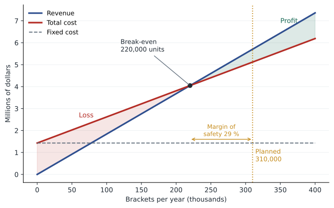
At 310,000 brackets, the line earns a profit of about 585,000 dollars with a margin of safety of about 29 %. Operating leverage of 3.4 means a 10 % change in volume moves profit by about a third. Daniel used this to argue for a long-term supply agreement with a minimum volume commitment: with high operating leverage, the risk is not the margin per bracket but a customer cutting orders.

Multiple products and sales mix

Most businesses sell many products with different contribution margins, so break-even depends on the sales mix. The usual approach computes a weighted average contribution margin per unit, or a weighted contribution margin ratio, using the expected mix, and divides fixed costs by it. A shift in mix toward lower-margin products raises the break-even point even if total sales are unchanged. Fairway watches mix constantly: a shopper who switches from fresh prepared foods, with a high contribution ratio, to discount staples, with a low one, can leave sales unchanged and cut profit.

Assumptions and limits of CVP

CVP analysis assumes that price, variable cost per unit and total fixed cost are constant over the relevant range, that the sales mix is constant, and that inventory levels do not change (so production equals sales). In reality, prices may need to fall to sell more, variable costs per unit may fall with volume discounts or rise with overtime, and fixed costs may step up. These assumptions do not make CVP useless; they mean it should be used for quick analysis within a sensible range and supported by sensitivity analysis. Running the model with a lower price, a higher variable cost and a lower volume, as the code above does for volume, shows which assumption matters most.

Kestrel provides a striking example. Its cost structure is almost all fixed: engineers, sales staff and office costs. Each additional subscription adds little variable cost beyond hosting and payment fees, so its contribution margin ratio is about 85 %. Leo showed that the company would break even at about 1,900 customers, compared with 1,450 today. Below that point it burns cash; above it, profit rises steeply. This is why software investors focus on growth: high operating leverage makes scale extraordinarily valuable, and lack of scale extraordinarily costly.

CVP in a service organization

Cost-volume-profit analysis is not limited to factories. Hana Kowalski used it at Lakeview Health to analyze a new evening clinic. The unit of volume was a patient visit. Variable costs per visit were small, mainly supplies and some fee-for-service physician payments, while nursing staff, rent, security and the scheduling system were fixed for the evening shift. With funding of about 85 dollars per visit and variable costs of about 22 dollars, each visit contributed about 63 dollars toward fixed costs of roughly 9,500 dollars a week, so the clinic needed about 150 visits a week to cover its costs.

The analysis also showed where the risks lay. Because most costs were fixed, operating leverage was high: a clinic running at 200 visits a week would generate a healthy surplus, but one running at 120 would lose money every week. Hana therefore recommended starting with three evenings rather than five, measuring demand for a quarter, and expanding only if volume passed the break-even level. In a not-for-profit setting the surplus is reinvested rather than distributed, but the logic of covering fixed costs is exactly the same as in a business.