
MATH-372 · Lesson 8 of 12 · 24 min
Integer programming and branch and bound
Many decisions are indivisible. A warehouse is opened or not, a crew is assigned to a flight or not, a truck makes a whole number of trips. Requiring some variables of a linear program to be integers gives an integer program, and this one change transforms the subject. The feasible set is no longer convex, the optimum need not be at a vertex of anything simple, and no algorithm is known that solves all integer programs efficiently. Yet integer programming is one of the great practical successes of optimization, because linear programming supplies bounds that let a systematic search discard most of the possibilities without examining them. This lesson shows how to model with integer and binary variables, why rounding fails, how branch and bound works and why it is correct, and why some integer programs, those with totally unimodular constraint matrices, are no harder than linear programs.
Modeling with integer variables
An integer program (IP) is a linear program with the extra requirement \(x_j \in \mathbb{Z}\) for some or all \(j\); when only some variables are integer it is a mixed-integer program (MIP). Binary variables, restricted to \(\{0, 1\}\), are especially expressive because they model yes-or-no decisions and logical conditions.
In the knapsack problem a hiker chooses among items with values \(v_i\) and weights \(w_i\), subject to a weight limit \(W\): maximize \(\sum v_ix_i\) subject to \(\sum w_ix_i \le W\), \(x_i \in \{0, 1\}\). It is the simplest integer program and appears inside larger models whenever a budget is allocated among indivisible projects.
A fixed charge models a setup cost. If producing \(x\) units costs \(f + cx\) when \(x > 0\) and nothing when \(x = 0\), introduce a binary \(z\) and write the cost as \(fz + cx\) with the constraint \(x \le Mz\), where \(M\) is an upper bound on production. If \(z = 0\), production is forced to zero; if \(z = 1\), the setup cost is paid and production is limited only by \(M\). Facility location models combine fixed charges for opening sites with transportation costs for serving customers from open sites.
Logical conditions become linear constraints on binaries. At most one of projects 1, 2, 3 is \(z_1 + z_2 + z_3 \le 1\); project 2 only if project 1 is \(z_2 \le z_1\). An either-or condition, \(a^Tx \le \alpha\) or \(d^Tx \le \beta\), uses one binary and big-\(M\) constants: \(a^Tx \le \alpha + Mz\) and \(d^Tx \le \beta + M(1 - z)\). The choice of \(M\) matters: it must be large enough not to cut off solutions, and as small as possible, because large \(M\) values weaken the LP relaxation discussed next.
LP relaxation and why rounding fails
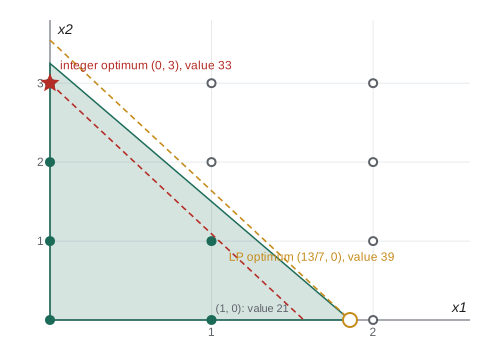
Dropping the integrality requirement gives the LP relaxation. Since every integer feasible point is feasible for the relaxation, the relaxation's optimal value bounds the integer optimum: for a maximization, \(z_{\text{IP}} \le z_{\text{LP}}\). If the relaxation's optimal solution happens to be integral, it solves the IP. Otherwise one might hope to round it. Consider
The relaxation's optimum is \(x = (\frac{13}{7}, 0)\) with value 39, since \(x_1\) has the better value per unit of the single resource (3 per unit versus 2.75). Rounding down gives \((1, 0)\) with value 21; rounding up is infeasible. The true integer optimum is \((0, 3)\) with value 33, which is nowhere near the relaxation's solution. In general the integer optimum can be arbitrarily far from the LP optimum, and rounded solutions can be infeasible or arbitrarily bad. Something more systematic is needed.
Branch and bound
Branch and bound, introduced by Ailsa Land and Alison Doig in 1960, organizes the search as a tree. Each node is a subproblem, the original IP with some extra bounds on variables. At each node we solve the LP relaxation. Then one of four things happens.
If the relaxation is infeasible, so is the subproblem, and the node is pruned. If the relaxation's value is no better than the best integer solution found so far, called the incumbent, no integer point in this subproblem can improve on it, and the node is pruned by bound. If the relaxation's solution is integral, it is the best integer point in the subproblem; it becomes the new incumbent if better, and the node is pruned. Otherwise some integer variable \(x_j\) has a fractional value \(\bar x_j\), and we branch: create two children, one with the extra constraint \(x_j \le \lfloor\bar x_j\rfloor\) and one with \(x_j \ge \lceil\bar x_j\rceil\). Every integer point of the parent lies in exactly one child, and the parent's fractional solution lies in neither.
Theorem. If the LP relaxation of a pure integer program has a bounded feasible set, branch and bound terminates, and the final incumbent is an optimal solution (or there is none, if no incumbent was found and the IP is infeasible).
Proof. Correctness: at every stage, the union of the integer feasible sets of the unprocessed nodes, together with the incumbent, contains every integer feasible point that could be better than the incumbent. This holds at the start (the root contains everything) and is preserved by each step: branching splits a node's integer points between its children without losing any, since an integer \(x_j\) satisfies \(x_j \le \lfloor\bar x_j\rfloor\) or \(x_j \ge \lceil\bar x_j\rceil\); pruning an infeasible node discards no integer points; pruning by bound discards only points no better than the incumbent; and pruning an integral node keeps its best point as a candidate incumbent. When no nodes remain, the incumbent is therefore optimal. Termination: the bounded relaxation means each variable ranges over finitely many integers. Each branching strictly shrinks the integer range of one variable in each child, so every path down the tree is finite, and since each node has at most two children, the tree is finite by König's lemma. \(\square\)
Two choices drive efficiency: which fractional variable to branch on, and which open node to process next. Depth-first search finds integer incumbents quickly, which enables pruning; best-bound search, which processes the node with the best relaxation value, minimizes the number of nodes needed to prove optimality. Modern solvers mix the two and add many refinements.
Worked problem
Reading the tree
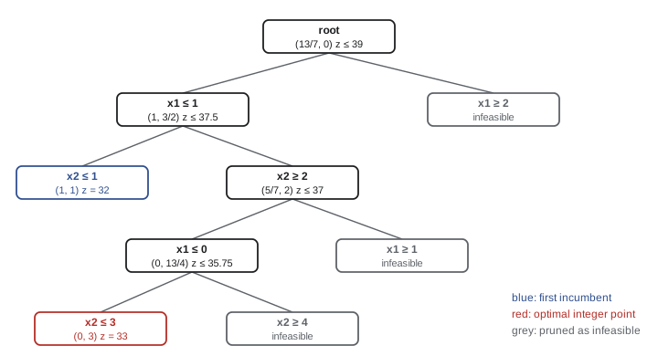
Follow branch and bound on \(\max 21x_1 + 11x_2\), \(7x_1 + 4x_2 \le 13\), \(x \ge 0\) integer, branching depth first on the down branch.
Show solution
- Root: relaxation \((\frac{13}{7}, 0)\), bound 39. Branch on \(x_1\): \(x_1 \le 1\) or \(x_1 \ge 2\).
- Node \(x_1 \le 1\): relaxation \((1, \frac32)\), bound 37.5. Branch on \(x_2\). Its child \(x_2 \le 1\) gives \((1, 1)\), integral with value 32: the first incumbent.
- Node \(x_1 \le 1,\ x_2 \ge 2\): relaxation \((\frac57, 2)\), bound 37 > 32, so branch on \(x_1\). The child \(x_1 \ge 1\) needs \(7 + 8 = 15 > 13\): infeasible. The child \(x_1 \le 0\) has relaxation \((0, \frac{13}{4})\), bound 35.75, and branches on \(x_2\): \(x_2 \le 3\) gives \((0, 3)\) with value 33, a better incumbent, and \(x_2 \ge 4\) is infeasible.
- Back at the root, \(x_1 \ge 2\) needs \(14 > 13\): infeasible. No open nodes remain.
Answer: The optimum is \((0, 3)\) with value 33. The gap between the root bound 39 and the optimum 33 is closed by nine LP solves, far fewer than one might fear, though for large problems the tree can grow exponentially.
The knapsack bound
For the knapsack problem the LP relaxation can be solved without the simplex method. Sort the items by value per unit weight, \(v_1/w_1 \ge v_2/w_2 \ge \cdots\), and fill the knapsack greedily, taking the first item that does not fit fractionally. George Dantzig observed in 1957 that this greedy fill is optimal for the relaxation.
Theorem. The greedy fractional solution solves the LP relaxation of the knapsack problem: maximize \(\sum v_ix_i\) subject to \(\sum w_ix_i \le W\), \(0 \le x_i \le 1\).
Proof. Let \(x\) be greedy and \(x'\) any feasible solution, and suppose without loss of generality that the total weight is \(W\) in both (if the items do not fill the knapsack, greedy takes everything and is clearly optimal). Greedy has \(x_i = 1\) for \(i < k\), \(x_i = 0\) for \(i > k\), and some \(x_k \in [0, 1]\). Let \(r = v_k/w_k\). For \(i < k\), \(x_i - x'_i \ge 0\) and \(v_i \ge rw_i\); for \(i > k\), \(x_i - x'_i \le 0\) and \(v_i \le rw_i\). So in every case \(v_i(x_i - x'_i) \ge rw_i(x_i - x'_i)\), and summing, \(\sum v_ix_i - \sum v_ix'_i \ge r(\sum w_ix_i - \sum w_ix'_i) \ge 0\), because greedy's weight is \(W\) and the other's is at most \(W\). \(\square\)
The bound is cheap, so knapsack branch and bound can explore many nodes quickly, and the greedy order suggests branching on the items in that order. The greedy integer solution, which skips items that do not fit, is often good but not optimal, as the program shows.
Totally unimodular problems
Some integer programs are secretly linear programs: their LP relaxations always have integral optimal vertices. A matrix is totally unimodular (TU) if every square submatrix has determinant \(0\), \(1\) or \(-1\).
Theorem. If \(A\) is totally unimodular and \(b\) is integral, every vertex of \(\{x : Ax \le b,\ x \ge 0\}\) is integral.
Proof. Stack \(A\) and \(-I\) into one constraint matrix; it is still TU, since a square submatrix involving rows of \(-I\) can be expanded along those rows, each with a single nonzero entry \(\pm1\), down to a square submatrix of \(A\). A vertex is the unique solution of \(Mx = d\) for some nonsingular \(n \times n\) submatrix \(M\) of the stacked matrix and the matching entries \(d\) of \((b, 0)\), as in lesson 3. By Cramer's rule \(x_j = \det M_j/\det M\), where \(M_j\) is \(M\) with column \(j\) replaced by \(d\). The denominator is \(\pm1\) and the numerator is an integer, so \(x_j\) is an integer. \(\square\)
The incidence matrix of a bipartite graph, with one row per vertex and one column per edge, is TU. This covers the transportation problem of lesson 2 and the assignment problem of matching \(n\) workers to \(n\) jobs at minimum cost, and more generally network flow problems. Solving their LP relaxations by the simplex method automatically gives integer solutions. This is why airlines could schedule crews and railways could route freight by linear programming long before general integer programming was practical.
Hardness and modern solvers
In 1972 Richard Karp listed 0-1 integer programming among his 21 NP-complete problems, so a polynomial algorithm for general integer programs would show P = NP. In practice, branch and bound is combined with cutting planes, extra linear inequalities satisfied by all integer points but violated by the current fractional solution, an idea introduced by Ralph Gomory in 1958. The combination, branch and cut, together with preprocessing, heuristics and very fast LP re-solves (a child's LP is warm-started from its parent's optimal basis by the dual simplex method), lets modern solvers handle many industrial problems with hundreds of thousands of integer variables. A practical measure of a model's quality is its integrality gap, the difference between the relaxation bound and the integer optimum: tighter formulations, such as smaller big-\(M\) constants, close the gap and shrink the tree.
Branch and bound in code
The program implements branch and bound for the two-variable example, using the exact two-phase simplex solver of lesson 6 for each relaxation and printing the tree, and checks the answer by brute force. It then solves a five-item knapsack by depth-first branch and bound with Dantzig's greedy bound, and checks it against all 32 subsets.
from fractions import Fraction as Fr

def solve_lp(c, A, b, sense):
    """Minimize c^T x subject to rows A[i] x (sense[i] in '<=', '>=', '=') b[i], x >= 0.
    Exact two-phase simplex with Bland's rule. Returns (status, x, value, y) where y holds
    the dual values (shadow prices) of the rows: y_i = d(optimal value)/d(b_i)."""
    m, n = len(A), len(c)
    rows, rhs, cols = [], [], n
    slack = {}
    for i in range(m):                                  # add slack or surplus columns
        r = [Fr(v) for v in A[i]]
        rows.append(r); rhs.append(Fr(b[i]))
        if sense[i] != '=':
            slack[i] = cols; cols += 1
    for i in range(m):
        rows[i] += [Fr(0)] * (cols - n)
        if i in slack:
            rows[i][slack[i]] = Fr(1 if sense[i] == '<=' else -1)
        if rhs[i] < 0:                                  # make the right side nonnegative
            rows[i] = [-v for v in rows[i]]; rhs[i] = -rhs[i]
    N = cols + m                                        # artificial columns cols .. cols+m-1
    T = [rows[i] + [Fr(int(k == i)) for k in range(m)] + [rhs[i]] for i in range(m)]
    basis = [cols + i for i in range(m)]

    def price(cost):
        z = [Fr(v) for v in cost] + [Fr(0)]
        for i, j in enumerate(basis):
            z = [a - z[j] * q for a, q in zip(z, T[i])]
        return z

    def pivot(r, e):
        p = T[r][e]
        T[r] = [v / p for v in T[r]]
        for i in range(len(T)):
            if i != r and T[i][e] != 0:
                f = T[i][e]; T[i] = [a - f * q for a, q in zip(T[i], T[r])]
        basis[r] = e

    def simplex(allowed):
        while True:
            e = next((j for j in allowed if T[-1][j] < 0), None)   # Bland: smallest index
            if e is None:
                return "optimal"
            rs = [i for i in range(len(T) - 1) if T[i][e] > 0]
            if not rs:
                return "unbounded"
            t = min(T[i][-1] / T[i][e] for i in rs)
            pivot(min((i for i in rs if T[i][-1] / T[i][e] == t), key=lambda i: basis[i]), e)

    T.append(price([0] * cols + [1] * m))               # phase one
    simplex(range(N))
    if T[-1][-1] != 0:
        return "infeasible", None, None, None
    T.pop()
    for i in range(m):                                  # drive zero artificials out if possible
        if basis[i] >= cols:
            e = next((j for j in range(cols) if T[i][j] != 0), None)
            if e is not None:
                pivot(i, e)
    T.append(price(list(c) + [0] * (cols - n) + [0] * m))
    status = simplex(range(cols))                       # phase two on original columns only
    if status != "optimal":
        return status, None, None, None
    x = [Fr(0)] * N
    for i, j in enumerate(basis):
        x[j] = T[i][-1]
    # duals from B^T y = c_B, read off the artificial columns: y = c_B^T B^{-1} (sign-corrected)
    y = [-T[-1][cols + i] for i in range(m)]
    y = [(-v if Fr(b[i]) < 0 else v) for i, v in enumerate(y)]
    return "optimal", x[:n], -T[-1][-1], y
import math
from itertools import product, combinations

# 1. branch and bound for: maximize 21 x1 + 11 x2  s.t.  7 x1 + 4 x2 <= 13,  x integer >= 0
c, A, b = [21, 11], [[7, 4]], [13]
best = {"value": None, "x": None}
nodes = []

def bb(bounds, depth, label):
    rows, rhs, sense = [r[:] for r in A], b[:], ["<="] * len(A)
    for j, (lo, hi) in enumerate(bounds):           # branching bounds become extra rows
        e = [int(k == j) for k in range(2)]
        if lo > 0: rows.append(e); rhs.append(lo); sense.append(">=")
        if hi is not None: rows.append(e); rhs.append(hi); sense.append("<=")
    st, x, v, _ = solve_lp([-ci for ci in c], rows, rhs, sense)
    pad = "   " * depth
    if st != "optimal":
        print(f"{pad}{label}: LP infeasible -> prune"); nodes.append(label); return
    z = -v
    nodes.append(label)
    text = f"{pad}{label}: LP x = ({x[0]}, {x[1]}), bound {z} = {float(z):.2f}"
    if best["value"] is not None and z <= best["value"]:
        print(text, "-> prune by bound"); return
    frac = [j for j in range(2) if x[j].denominator != 1]
    if not frac:
        best["value"], best["x"] = z, x
        print(text, "-> integer: new incumbent"); return
    j = frac[0]
    print(text, f"-> branch on x{j + 1}")
    lo, hi = bounds[j]
    down = list(bounds); down[j] = (lo, math.floor(x[j]))
    up = list(bounds); up[j] = (math.ceil(x[j]), hi)
    bb(down, depth + 1, f"x{j + 1} <= {math.floor(x[j])}")
    bb(up, depth + 1, f"x{j + 1} >= {math.ceil(x[j])}")

bb([(0, None), (0, None)], 0, "root")
print(f"optimum x = ({best['x'][0]}, {best['x'][1]}), value {best['value']}; {len(nodes)} nodes")
brute = max((21 * p + 11 * q, (p, q)) for p, q in product(range(3), range(5)) if 7 * p + 4 * q <= 13)
print("brute force check:", brute)

# 2. 0-1 knapsack by depth-first branch and bound with Dantzig's fractional bound
val = [40, 42, 25, 12, 30]
wt = [4, 7, 5, 3, 6]
cap = 15
order = sorted(range(5), key=lambda i: -val[i] / wt[i])   # best value per unit weight first

def bound(k, room, v):
    """LP relaxation of the remaining items: fill greedily, take a fraction of the first misfit."""
    for i in order[k:]:
        if wt[i] <= room:
            room -= wt[i]; v += val[i]
        else:
            return v + Fr(val[i] * room, wt[i])
    return Fr(v)

count = [0]
def knap(k, room, v, chosen, inc):
    count[0] += 1
    if k == len(order):
        return (v, chosen) if v > inc[0] else inc
    if bound(k, room, v) <= inc[0]:
        return inc                                    # cannot beat the incumbent
    i = order[k]
    if wt[i] <= room:
        inc = knap(k + 1, room - wt[i], v + val[i], chosen + [i + 1], inc)
    return knap(k + 1, room, v, chosen, inc)

v, items = knap(0, cap, 0, [], (0, []))
print(f"knapsack: root bound {bound(0, cap, 0)}, optimum {v} with items {sorted(items)}, {count[0]} nodes visited")
allsets = max((sum(val[i] for i in S), S) for r in range(6) for S in combinations(range(5), r)
              if sum(wt[i] for i in S) <= cap)
print("all 32 subsets checked:", allsets[0], [i + 1 for i in allsets[1]])root: LP x = (13/7, 0), bound 39 = 39.00 -> branch on x1
x1 <= 1: LP x = (1, 3/2), bound 75/2 = 37.50 -> branch on x2
x2 <= 1: LP x = (1, 1), bound 32 = 32.00 -> integer: new incumbent
x2 >= 2: LP x = (5/7, 2), bound 37 = 37.00 -> branch on x1
x1 <= 0: LP x = (0, 13/4), bound 143/4 = 35.75 -> branch on x2
x2 <= 3: LP x = (0, 3), bound 33 = 33.00 -> integer: new incumbent
x2 >= 4: LP infeasible -> prune
x1 >= 1: LP infeasible -> prune
x1 >= 2: LP infeasible -> prune
optimum x = (0, 3), value 33; 9 nodes
brute force check: (33, (0, 3))
knapsack: root bound 102, optimum 95 with items [1, 3, 5], 14 nodes visited
all 32 subsets checked: 95 [1, 3, 5]The tree matches the hand computation: nine nodes, with the first incumbent 32 improved to the optimum 33. For the knapsack, the root bound is 102 (items 1 and 2 plus four fifths of item 3), the greedy integer fill would take items 1, 2 and 4 for a value of 94, and branch and bound finds the true optimum 95 with items 1, 3 and 5, filling the 15 kg exactly, after visiting 14 nodes of the 63 in the full binary tree.
Common mistakes
MistakeRounding the LP solution and calling it optimal.
InsteadRounded points can be infeasible or far from optimal; the LP value is only a bound.
MistakePruning a node whose LP bound equals the incumbent value, and then claiming every optimum has been found.
InsteadPruning at equality is correct for finding one optimum, but alternative optima in that node are discarded.
MistakeUsing a huge big-M constant to be safe.
InsteadLarge \(M\) weakens the relaxation and enlarges the search tree; use the smallest valid bound.
MistakeBranching with \(x_j \le \bar x_j\) and \(x_j \ge \bar x_j\).
InsteadBranch on \(x_j \le \lfloor\bar x_j\rfloor\) and \(x_j \ge \lceil\bar x_j\rceil\) to exclude the fractional point.
MistakeAssuming all integer programs are hard.
InsteadTotally unimodular problems, including transportation and assignment, have integral LP optima.
Summary and key terms
- Integer and binary variables model indivisibility, fixed charges and logical conditions; big-M constraints link them to continuous variables.
- The LP relaxation bounds the integer optimum, but rounding its solution can fail badly.
- Branch and bound (Land and Doig, 1960) solves relaxations on a tree, branching on fractional variables and pruning by infeasibility, bound or integrality.
- For bounded pure IPs, branch and bound terminates with an optimal solution.
- The knapsack relaxation is solved by Dantzig's greedy fill by value per unit weight.
- Totally unimodular constraint matrices, such as bipartite incidence matrices, give integral LP vertices.
- integer program
- A linear program in which some or all variables must take integer values.
- LP relaxation
- The linear program obtained by dropping integrality requirements.
- incumbent
- The best integer feasible solution found so far in a search.
- branching
- Splitting a subproblem by adding complementary bounds on a fractional variable.
- pruning by bound
- Discarding a subproblem whose relaxation value cannot beat the incumbent.
- totally unimodular
- A matrix all of whose square submatrices have determinant 0, 1 or −1.
- integrality gap
- The difference between the LP relaxation bound and the integer optimum.
Practice problems
Work each problem on paper first, then reveal the answer to check.
Model: produce \(x\) units at 4 dollars each plus a setup cost of 100 if \(x > 0\), with capacity 50.
Show answer
Cost \(100z + 4x\) with \(0 \le x \le 50z\), \(z \in \{0, 1\}\).
Model the condition that \(x_1 + x_2 \le 4\) or \(x_1 - x_2 \ge 2\), given \(0 \le x_1, x_2 \le 10\).
Show answer
\(x_1 + x_2 \le 4 + 16z\) and \(x_1 - x_2 \ge 2 - 12(1 - z)\), \(z \in \{0, 1\}\); 16 and 12 are the largest possible violations.
Solve \(\max 5x_1 + 4x_2\) s.t. \(6x_1 + 4x_2 \le 24\), \(x_1 + 2x_2 \le 6\), integer \(x \ge 0\), with branch and bound.
Show answer
The relaxation optimum is \((3, 1.5)\), value 21. Branch \(x_2 \le 1\): relaxation \((\frac{10}{3}, 1)\), value \(20.67\); branch \(x_2 \ge 2\): relaxation \((2, 2)\), value 18, integral. Under \(x_2 \le 1\), \(x_1 \le 3\) gives \((3, 1)\), value 19, and \(x_1 \ge 4\) gives \((4, 0)\), value 20. The optimum is \((4, 0)\) with value 20.
Why is the root LP bound of a maximization IP at least the IP optimum?
Show answer
The IP feasible set is contained in the LP feasible set, and a maximum over a larger set is at least as large.
Show that \(\begin{pmatrix} 1 & 1 & 0 \\ 0 & 1 & 1 \\ 1 & 0 & 1 \end{pmatrix}\) is not totally unimodular.
Show answer
Its determinant is \(1(1 - 0) - 1(0 - 1) + 0 = 2\).
For the knapsack with values 60, 100, 120, weights 10, 20, 30 and capacity 50, find the LP bound and the integer optimum.
Show answer
Ratios 6, 5, 4: the bound takes items 1 and 2 and two thirds of item 3, value 240. The integer optimum takes items 2 and 3, value 220.
Lesson quiz · 5 questions
Score 60% or more to complete this lesson.
Create a free account to save your progress, take quizzes and earn a certificate.