Unconstrained optimization: gradient descent and Newton's method

Most smooth optimization algorithms rest on two simple ideas: walk downhill, and model the function locally by something you can minimize exactly. Gradient descent, proposed by Augustin-Louis Cauchy in 1847 for solving systems of equations arising in astronomy, follows the first idea with a linear model; Newton's method follows the second with a quadratic model. This lesson treats the unconstrained problem of minimizing a smooth function \(f : \mathbb{R}^n \to \mathbb{R}\). It first proves the optimality conditions that any method aims to satisfy, then develops line searches, proves convergence results for gradient descent, explains its slowness on ill-conditioned problems, and shows why Newton's method converges so fast near a minimizer.

Optimality conditions

Let \(f\) be twice continuously differentiable. Taylor's theorem says that for a direction \(h\) and some \(\theta \in (0, 1)\),

Theorem (necessary conditions). If \(x^*\) is a local minimizer of \(f\), then \(\nabla f(x^*) = 0\) and \(\nabla^2f(x^*)\) is positive semidefinite.

Proof. If \(g = \nabla f(x^*) \ne 0\), then \(\frac{d}{dt}f(x^* - tg)\big|_{t=0} = -\|g\|^2 < 0\), so \(f(x^* - tg) < f(x^*)\) for small \(t > 0\), contradicting local minimality. With \(\nabla f(x^*) = 0\), if some \(v\) had \(v^T\nabla^2f(x^*)v < 0\), then by continuity \(v^T\nabla^2f(x^* + \theta tv)v < 0\) for small \(t\), and Taylor's formula gives \(f(x^* + tv) = f(x^*) + \frac{t^2}{2}v^T\nabla^2f(x^* + \theta tv)v < f(x^*)\): again a contradiction. \(\square\)

Theorem (sufficient conditions). If \(\nabla f(x^*) = 0\) and \(\nabla^2f(x^*)\) is positive definite, then \(x^*\) is a strict local minimizer.

Proof. Positive definiteness is preserved under small perturbations (the smallest eigenvalue is continuous), so \(\nabla^2f\) is positive definite on a ball around \(x^*\). For \(h \ne 0\) small enough that \(x^* + h\) is in the ball, Taylor's formula gives \(f(x^* + h) = f(x^*) + \frac12h^T\nabla^2f(x^* + \theta h)h > f(x^*)\). \(\square\)

There is a gap between the two theorems: \(x^3\) at 0 satisfies the necessary conditions without being a minimizer, and \(x^4\) at 0 is a minimizer that fails the sufficient ones. For convex functions the gap closes completely, since by lesson 9 a stationary point is a global minimizer. Numerical methods look for stationary points, and in nonconvex problems they usually find local minimizers, because saddle points and maxima are unstable for descent methods.

Descent directions and line searches

An iterative method generates \(x_{k+1} = x_k + t_kd_k\) with a direction \(d_k\) and a step length \(t_k > 0\). The direction is a descent direction if \(\nabla f(x_k)^Td_k < 0\), so that \(f\) decreases for small enough steps. The steepest descent direction is \(d = -\nabla f(x)\), which minimizes the directional derivative \(\nabla f^Td\) over unit vectors by the Cauchy–Schwarz inequality.

Choosing the step length well matters as much as the direction. Too long a step can increase \(f\); too short a step wastes iterations. Exact minimization along the line is rarely worth its cost. Instead, practical methods accept any step giving sufficient decrease, the Armijo condition of 1966:

Backtracking line search starts with \(t = 1\) and multiplies \(t\) by a factor \(\beta \in (0, 1)\), often \(\frac12\), until the Armijo condition holds. It always stops: \(f(x + td) = f(x) + t\nabla f(x)^Td + o(t)\), and because \(\nabla f(x)^Td < 0\) and \(\alpha < 1\), the right side of the Armijo condition exceeds \(f(x + td)\) once \(t\) is small. The condition with a small \(\alpha\) such as \(10^{-4}\) asks only for a decrease proportional to what the linear model predicts.

Convergence of gradient descent

A function has an \(L\)-Lipschitz gradient, or is \(L\)-smooth, if \(\|\nabla f(x) - \nabla f(y)\| \le L\|x - y\|\) for all \(x, y\). For twice differentiable \(f\) this means the eigenvalues of the Hessian lie in \([-L, L]\).

Lemma (descent lemma). If \(f\) is \(L\)-smooth, then \(f(y) \le f(x) + \nabla f(x)^T(y - x) + \frac L2\|y - x\|^2\) for all \(x, y\).

Proof. By the fundamental theorem of calculus along the segment, \(f(y) - f(x) - \nabla f(x)^T(y - x) = \int_0^1 (\nabla f(x + s(y - x)) - \nabla f(x))^T(y - x)\,ds\). By Cauchy–Schwarz and the Lipschitz condition the integrand is at most \(Ls\|y - x\|^2\), and \(\int_0^1 Ls\,ds = \frac L2\). \(\square\)

Taking \(y = x - t\nabla f(x)\) with \(0 < t \le 1/L\) gives \(f(y) \le f(x) - t(1 - \frac{Lt}{2})\|\nabla f(x)\|^2 \le f(x) - \frac t2\|\nabla f(x)\|^2\). Each step decreases \(f\) by an amount proportional to the squared gradient.

Theorem. Let \(f\) be \(L\)-smooth and bounded below by \(f^*\), and run gradient descent with constant step \(t = 1/L\). Then \(\min_{0 \le k < K}\|\nabla f(x_k)\|^2 \le 2L(f(x_0) - f^*)/K\). If in addition \(f\) is convex with a minimizer \(x^*\), then \(f(x_K) - f(x^*) \le L\|x_0 - x^*\|^2/(2K)\).

Proof. Summing the decrease estimate \(f(x_{k+1}) \le f(x_k) - \frac{1}{2L}\|\nabla f(x_k)\|^2\) over \(k < K\) telescopes to \(\frac{1}{2L}\sum_{k<K}\|\nabla f(x_k)\|^2 \le f(x_0) - f(x_K) \le f(x_0) - f^*\), and the minimum is at most the average. For the convex case write \(g = \nabla f(x_k)\) and \(t = 1/L\). Convexity gives \(f(x_k) \le f(x^*) + g^T(x_k - x^*)\), so \(f(x_{k+1}) \le f(x^*) + g^T(x_k - x^*) - \frac t2\|g\|^2 = f(x^*) + \frac{1}{2t}\big(\|x_k - x^*\|^2 - \|x_k - tg - x^*\|^2\big)\), by expanding the square. The last norm is \(\|x_{k+1} - x^*\|\), so the sum over \(k < K\) telescopes: \(\sum_{k<K}(f(x_{k+1}) - f(x^*)) \le \frac{1}{2t}\|x_0 - x^*\|^2\). Since \(f(x_k)\) decreases, the last term is the smallest, and \(K(f(x_K) - f(x^*)) \le \frac L2\|x_0 - x^*\|^2\). \(\square\)

If \(f\) is also \(\mu\)-strongly convex, meaning \(\nabla^2f \succeq \mu I\), the convergence is linear: \(f(x_k) - f^* \le (1 - \mu/L)^k(f(x_0) - f^*)\). The ratio \(\kappa = L/\mu\) is the condition number, and the number of iterations needed for a given accuracy grows in proportion to \(\kappa\). Yurii Nesterov showed in 1983 that a clever use of momentum reduces this to \(\sqrt\kappa\), which is optimal for methods using only gradients.

The zigzag

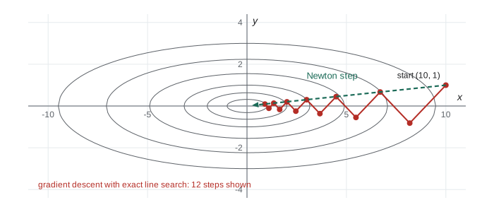
Why does conditioning matter so much? Take \(f(x, y) = \frac12(x^2 + \kappa y^2)\). Its level sets are ellipses elongated by a factor \(\sqrt\kappa\) along the \(x\) axis. The gradient \((x, \kappa y)\) is perpendicular to the level curve, which for a long thin ellipse points almost straight across the valley rather than along it toward the minimizer. Even with exact line searches, each step overshoots across the valley and the next one comes back, and the error in \(f\) can shrink by as little as \(\big(\frac{\kappa - 1}{\kappa + 1}\big)^2\) per step, a bound that follows from an inequality of Kantorovich. For \(\kappa = 100\) that is about 0.96, so it can take about 290 steps to gain a factor of \(10^5\) in accuracy.

Newton's method

Newton's method replaces \(f\) near \(x_k\) by its second-order Taylor model \(m(h) = f(x_k) + \nabla f(x_k)^Th + \frac12h^T\nabla^2f(x_k)h\). If the Hessian is positive definite, \(m\) is a strictly convex quadratic with minimizer given by the Newton equation

Equivalently, Newton's method for optimization is Newton's root-finding method, published by Isaac Newton and Joseph Raphson in the late seventeenth century, applied to the equation \(\nabla f(x) = 0\). The Newton direction is a descent direction when the Hessian is positive definite, since \(\nabla f^Th = -\nabla f^T(\nabla^2f)^{-1}\nabla f < 0\). For a strictly convex quadratic, the model is exact and one step lands on the minimizer from anywhere, regardless of conditioning. More generally, Newton's method is affine invariant: changing variables by \(x = Ay\) transforms the iterates in exactly the same way, so it is unaffected by the scaling that cripples gradient descent.

Theorem (local quadratic convergence). Suppose \(\nabla f(x^*) = 0\), \(\nabla^2f\) is Lipschitz with constant \(M\) near \(x^*\), and \(\|\nabla^2f(x)^{-1}\| \le 1/\mu\) for all \(x\) near \(x^*\). Then for \(x_k\) close to \(x^*\), the Newton step satisfies \(\|x_{k+1} - x^*\| \le \frac{M}{2\mu}\|x_k - x^*\|^2\).

Proof. Write \(H = \nabla^2f(x_k)\) and \(e = x_k - x^*\). Since \(\nabla f(x^*) = 0\), \(x_{k+1} - x^* = e - H^{-1}\nabla f(x_k) = H^{-1}\big(He - (\nabla f(x_k) - \nabla f(x^*))\big)\). By the fundamental theorem of calculus, \(\nabla f(x_k) - \nabla f(x^*) = \int_0^1 \nabla^2f(x^* + se)e\,ds\), so \(x_{k+1} - x^* = H^{-1}\int_0^1 \big(\nabla^2f(x_k) - \nabla^2f(x^* + se)\big)e\,ds\). The Lipschitz condition bounds the integrand by \(M(1 - s)\|e\|^2\), whose integral is \(\frac M2\|e\|^2\), and \(\|H^{-1}\| \le 1/\mu\). \(\square\)

Once \(\|x_k - x^*\| < \mu/M\), the error is squared at each step, roughly doubling the number of correct digits per iteration: errors of \(10^{-2}\), \(10^{-4}\), \(10^{-8}\), \(10^{-16}\). Far from the minimizer, however, the pure Newton step can increase \(f\), head to a saddle point or a maximum, or be undefined when the Hessian is singular. Damped Newton adds a backtracking line search on the Newton direction, falling back on the gradient if the Newton direction is not a descent direction, and switches to full steps automatically once they satisfy the Armijo condition near the minimizer. The price of Newton's method is forming and solving with the Hessian, about \(n^3/3\) operations per step for a dense problem. Quasi-Newton methods, above all the BFGS method found independently by Broyden, Fletcher, Goldfarb and Shanno in 1970, build up a Hessian approximation from gradient differences and keep much of the speed at a fraction of the cost.

Gradient descent and Newton in code

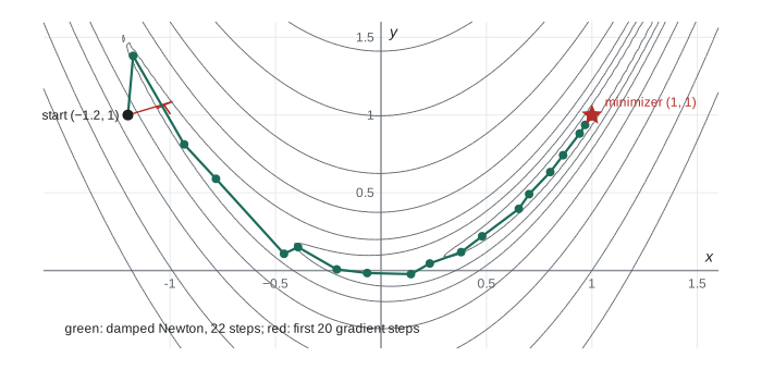
The program implements gradient descent and damped Newton, both with Armijo backtracking. It first runs them on the quadratic \(\frac12(x^2 + \kappa y^2)\) for condition numbers from 1 to 1000, then on the Rosenbrock function \((1 - x)^2 + 100(y - x^2)^2\) from the classic starting point \((-1.2, 1)\) proposed by Howard Rosenbrock in 1960, printing every Newton iterate.

import math

def backtracking(f, x, g, d, t=1.0, alpha=1e-4, beta=0.5):
    """Armijo backtracking: shrink t until f(x + t d) <= f(x) + alpha t g.d"""
    fx, slope = f(x), sum(gi * di for gi, di in zip(g, d))
    while f([xi + t * di for xi, di in zip(x, d)]) > fx + alpha * t * slope:
        t *= beta
    return t

def gradient_descent(f, grad, x, tol=1e-8, maxit=100000):
    for k in range(maxit):
        g = grad(x)
        if math.hypot(*g) < tol:
            return x, k
        d = [-gi for gi in g]
        t = backtracking(f, x, g, d)
        x = [xi + t * di for xi, di in zip(x, d)]
    return x, maxit

def newton(f, grad, hess, x, tol=1e-10, maxit=100, log=False):
    for k in range(maxit):
        g = grad(x)
        if math.hypot(*g) < tol:
            return x, k
        (a, b), (c, d_) = hess(x)
        det = a * d_ - b * c
        step = [-(d_ * g[0] - b * g[1]) / det, -(-c * g[0] + a * g[1]) / det]   # solve H p = -g
        if sum(gi * si for gi, si in zip(g, step)) >= 0:                         # not a descent direction
            step = [-gi for gi in g]
        t = backtracking(f, x, g, step)
        x = [xi + t * si for xi, si in zip(x, step)]
        if log:
            print(f"   Newton iter {k + 1:2d}: t = {t:<6g} x = ({x[0]:+.10f}, {x[1]:+.10f}), |grad| = {math.hypot(*grad(x)):.2e}")
    return x, maxit

# 1. ill-conditioned quadratic f = (x^2 + kappa y^2)/2: gradient descent slows as kappa grows
for kappa in (1, 10, 100, 1000):
    f = lambda v, k=kappa: 0.5 * (v[0] ** 2 + k * v[1] ** 2)
    grad = lambda v, k=kappa: [v[0], k * v[1]]
    hess = lambda v, k=kappa: ((1.0, 0.0), (0.0, float(k)))
    _, kg = gradient_descent(f, grad, [1.0, 1.0])
    _, kn = newton(f, grad, hess, [1.0, 1.0])
    print(f"quadratic, condition number {kappa:4d}: gradient descent {kg:5d} iterations, Newton {kn}")

# 2. Rosenbrock's banana from the classic start (-1.2, 1)
f = lambda v: (1 - v[0]) ** 2 + 100 * (v[1] - v[0] ** 2) ** 2
grad = lambda v: [-2 * (1 - v[0]) - 400 * v[0] * (v[1] - v[0] ** 2), 200 * (v[1] - v[0] ** 2)]
hess = lambda v: ((2 - 400 * v[1] + 1200 * v[0] ** 2, -400 * v[0]), (-400 * v[0], 200.0))
x, k = gradient_descent(f, grad, [-1.2, 1.0], tol=1e-6)
print(f"Rosenbrock, gradient descent: {k} iterations to |grad| < 1e-6, x = ({x[0]:.6f}, {x[1]:.6f})")
print("Rosenbrock, damped Newton:")
x, k = newton(f, grad, hess, [-1.2, 1.0], log=True)
print(f"   converged in {k} iterations to ({x[0]:.12f}, {x[1]:.12f})")

quadratic, condition number    1: gradient descent     1 iterations, Newton 1
quadratic, condition number   10: gradient descent    74 iterations, Newton 1
quadratic, condition number  100: gradient descent   840 iterations, Newton 1
quadratic, condition number 1000: gradient descent  9243 iterations, Newton 1
Rosenbrock, gradient descent: 13756 iterations to |grad| < 1e-6, x = (0.999999, 0.999998)
Rosenbrock, damped Newton:
   Newton iter  1: t = 1      x = (-1.1752808989, +1.3806741573), |grad| = 4.64e+00
   Newton iter  2: t = 0.125  x = (-0.9329814276, +0.8112106558), |grad| = 2.86e+01
   Newton iter  3: t = 1      x = (-0.7825400790, +0.5897363758), |grad| = 1.16e+01
   Newton iter  4: t = 1      x = (-0.4599971191, +0.1075633886), |grad| = 3.03e+01
   Newton iter  5: t = 1      x = (-0.3930456341, +0.1500023692), |grad| = 3.60e+00
   Newton iter  6: t = 0.25   x = (-0.2094119091, +0.0067701267), |grad| = 9.25e+00
   Newton iter  7: t = 1      x = (-0.0657190214, -0.0163286562), |grad| = 4.92e+00
   Newton iter  8: t = 1      x = (+0.1420425452, -0.0229887839), |grad| = 8.66e+00
   Newton iter  9: t = 1      x = (+0.2311071976, +0.0454780245), |grad| = 1.78e+00
   Newton iter 10: t = 0.5    x = (+0.3797428192, +0.1181458046), |grad| = 5.88e+00
   Newton iter 11: t = 1      x = (+0.4795948897, +0.2200408222), |grad| = 2.18e+00
   Newton iter 12: t = 1      x = (+0.6534058298, +0.3967289355), |grad| = 9.40e+00
   Newton iter 13: t = 1      x = (+0.7026236343, +0.4912575792), |grad| = 4.92e-01
   Newton iter 14: t = 0.5    x = (+0.8027855344, +0.6332210119), |grad| = 3.92e+00
   Newton iter 15: t = 1      x = (+0.8634908081, +0.7419312454), |grad| = 1.24e+00
   Newton iter 16: t = 1      x = (+0.9420786864, +0.8813361968), |grad| = 2.53e+00
   Newton iter 17: t = 1      x = (+0.9679918175, +0.9363366683), |grad| = 2.38e-01
   Newton iter 18: t = 1      x = (+0.9962103108, +0.9916386999), |grad| = 3.48e-01
   Newton iter 19: t = 1      x = (+0.9994793791, +0.9989483424), |grad| = 3.87e-03
   Newton iter 20: t = 1      x = (+0.9999988896, +0.9999975093), |grad| = 1.19e-04
   Newton iter 21: t = 1      x = (+0.9999999999, +0.9999999999), |grad| = 4.47e-10
   Newton iter 22: t = 1      x = (+1.0000000000, +1.0000000000), |grad| = 0.00e+00
   converged in 22 iterations to (1.000000000000, 1.000000000000)

On the quadratics, Newton needs a single step whatever the conditioning, while gradient descent needs roughly ten times as many iterations each time \(\kappa\) grows tenfold, as the linear-rate theory predicts. On the Rosenbrock function, gradient descent needs more than ten thousand iterations to reduce the gradient below \(10^{-6}\), creeping along the curved valley. Damped Newton takes about twenty iterations, cutting the step in several early ones where the quadratic model is poor, and then the last few lines show the signature of quadratic convergence: the gradient norm falls from about \(4 \times 10^{-3}\) to \(10^{-4}\) to \(5 \times 10^{-10}\) and then to zero in floating point, each step roughly squaring the previous error.