Constrained optimization: Lagrange multipliers and KKT conditions

When constraints are present, the minimizer usually sits on the boundary of the feasible set, where the gradient of the objective does not vanish. What replaces the condition \(\nabla f = 0\)? For equality constraints the answer goes back to Joseph-Louis Lagrange, who introduced multipliers in his Mécanique analytique of 1788: at a constrained optimum the gradient of the objective is a combination of the gradients of the constraints. For inequality constraints the answer is the Karush–Kuhn–Tucker (KKT) conditions, found by William Karush in his 1939 master's thesis at the University of Chicago and independently by Harold Kuhn and Albert Tucker, who published them in 1951. This lesson develops both, explains the constraint qualifications they need, proves that the KKT conditions are sufficient for convex problems, and shows that linear programming duality and complementary slackness are the KKT conditions in a special case.

Equality constraints and Lagrange multipliers

Consider minimizing \(f(x)\) subject to \(h(x) = 0\) for a single smooth constraint in \(\mathbb{R}^n\). At a point \(x^*\) of the constraint surface, the directions in which we can move while staying on the surface, to first order, are the tangent directions \(d\) with \(\nabla h(x^*)^Td = 0\). If \(x^*\) is a local minimizer, \(f\) cannot decrease to first order along any tangent direction, so \(\nabla f(x^*)^Td = 0\) for every \(d\) orthogonal to \(\nabla h(x^*)\). That forces \(\nabla f(x^*)\) to be parallel to \(\nabla h(x^*)\): \(\nabla f(x^*) + \lambda\nabla h(x^*) = 0\) for some number \(\lambda\), the Lagrange multiplier. In pictures, the level set of \(f\) through \(x^*\) is tangent to the constraint surface.

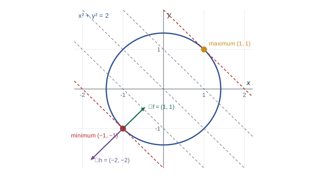
With several equality constraints \(h_1(x) = \cdots = h_p(x) = 0\), the same reasoning needs one more ingredient: the tangent directions must really be the directions \(d\) with \(\nabla h_j(x^*)^Td = 0\) for all \(j\). This holds when the constraint gradients are linearly independent at \(x^*\), the linear independence constraint qualification (LICQ), by the implicit function theorem: the constraint set is then a smooth surface of dimension \(n - p\) near \(x^*\), and every vector in the null space of the constraint Jacobian is the velocity of a smooth curve in the surface.

Theorem (Lagrange). Let \(x^*\) be a local minimizer of \(f\) subject to \(h_j(x) = 0\), \(j = 1, \ldots, p\), with \(f\) and \(h_j\) continuously differentiable and the gradients \(\nabla h_j(x^*)\) linearly independent. Then there are unique multipliers \(\lambda_1, \ldots, \lambda_p\) with

Proof sketch. Let \(d\) satisfy \(\nabla h_j(x^*)^Td = 0\) for all \(j\). By the implicit function theorem there is a smooth curve \(x(t)\) in the constraint set with \(x(0) = x^*\) and \(x'(0) = d\). Since \(t = 0\) is a local minimum of \(f(x(t))\), its derivative \(\nabla f(x^*)^Td\) is zero. So \(\nabla f(x^*)\) is orthogonal to the null space of the Jacobian, which means it lies in the row space, spanned by the \(\nabla h_j(x^*)\). Independence makes the coefficients unique. \(\square\)

The Lagrangian \(L(x, \lambda) = f(x) + \sum_j\lambda_jh_j(x)\) packages the conditions neatly: \(\nabla_xL = 0\) and \(\nabla_\lambda L = h(x) = 0\) together give \(n + p\) equations in \(n + p\) unknowns. Solving them gives candidates, which must then be compared or tested with second-order conditions, since maxima satisfy the same equations. The second-order test uses the Hessian of the Lagrangian restricted to tangent directions: if \(d^T\nabla^2_{xx}L(x^*, \lambda)d > 0\) for every nonzero tangent \(d\), the candidate is a strict local minimizer.

Multipliers measure sensitivity, as shadow prices did in lesson 7. If the constraint is changed to \(h(x) = u\) and the optimal value is \(p^*(u)\), then under the conditions of the theorem and a second-order condition, \(\frac{dp^*}{du}(0) = -\lambda\). In the circle example, enlarging the circle to \(x^2 + y^2 = 2 + u\) moves the minimizer outward to \(-\sqrt{(2 + u)/2}\,(1, 1)\), and \(p^*(u) = -\sqrt{4 + 2u}\), whose derivative at 0 is \(-\frac12 = -\lambda\).

Inequality constraints and the KKT conditions

Now consider the general problem of lesson 1, minimize \(f(x)\) subject to \(g_i(x) \le 0\) (\(i = 1, \ldots, m\)) and \(h_j(x) = 0\) (\(j = 1, \ldots, p\)). An inequality constraint that is slack at \(x^*\) does not restrict small moves and should play no role, while an active one, \(g_i(x^*) = 0\), acts like an equality constraint that can be released in one direction. The KKT conditions express this: there are multipliers \(\mu_i\) and \(\lambda_j\) with

Complementary slackness kills the multipliers of slack constraints. The sign condition \(\mu_i \ge 0\) is the new feature: stationarity says \(-\nabla f(x^*) = \sum\mu_i\nabla g_i(x^*) + \sum\lambda_j\nabla h_j(x^*)\), so with no equality constraints the negative gradient, the direction of steepest descent, lies in the cone spanned by the outward normals of the active constraints. Any move that would decrease \(f\) would push outward through some active constraint. If some \(\mu_i\) were negative, releasing constraint \(i\), that is moving into the interior, would decrease \(f\), and the point would not be optimal.

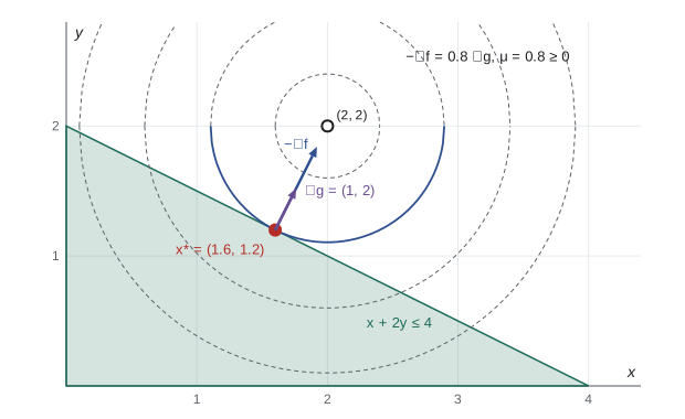
Theorem (KKT necessary conditions). Let \(x^*\) be a local minimizer at which a constraint qualification holds, for instance LICQ: the gradients of the active inequality constraints and of the equality constraints are linearly independent. Then there exist multipliers satisfying the KKT conditions.

Proof sketch. Let \(A\) be the set of active inequality constraints. Under the constraint qualification, every direction \(d\) with \(\nabla g_i(x^*)^Td < 0\) for \(i \in A\) and \(\nabla h_j(x^*)^Td = 0\) for all \(j\) is the initial velocity of a feasible curve, by the implicit function theorem applied to the equalities, together with the fact that strictly decreasing active constraints and slack inactive ones stay feasible for a while. At a local minimizer \(f\) cannot decrease along such a curve, so no such \(d\) has \(\nabla f(x^*)^Td < 0\). The same holds for directions with \(\nabla g_i(x^*)^Td \le 0\): by LICQ there is \(\bar d\) with \(\nabla g_i(x^*)^T\bar d = -1\) for \(i \in A\) and \(\nabla h_j(x^*)^T\bar d = 0\), and if such a \(d\) had \(\nabla f(x^*)^Td < 0\), then \(d + \varepsilon\bar d\) for small \(\varepsilon > 0\) would be a strict direction of the previous kind with \(\nabla f(x^*)^T(d + \varepsilon\bar d) < 0\). So the system \(\nabla f(x^*)^Td < 0\), \(\nabla g_i(x^*)^Td \le 0\) (\(i \in A\)), \(\nabla h_j(x^*)^Td = 0\) has no solution. Writing the equalities as pairs of inequalities, Farkas's lemma of lesson 6 (in the form: either \(c^Td < 0\) and \(Gd \le 0\) has a solution, or \(-c = G^T\mu\) for some \(\mu \ge 0\)) gives nonnegative multipliers \(\mu_i\), \(i \in A\), and free \(\lambda_j\) with \(-\nabla f(x^*) = \sum_{i \in A}\mu_i\nabla g_i(x^*) + \sum_j\lambda_j\nabla h_j(x^*)\). Setting \(\mu_i = 0\) for the inactive constraints gives complementary slackness. \(\square\)

Constraint qualifications cannot simply be dropped. Minimize \(x\) subject to \(x^2 \le 0\). The only feasible point is \(x = 0\), so it is the minimizer. But \(\nabla f = 1\) and \(\nabla g = 2x = 0\) there, so stationarity \(1 + \mu \cdot 0 = 0\) is impossible: no multiplier exists. The constraint gradient vanishes, LICQ fails, and the linearized constraints (any \(d\) satisfies \(0 \cdot d \le 0\)) describe a much larger set than the true feasible set. Besides LICQ, common qualifications are that all constraints are affine, which is why LP needs none, and, for convex problems, Slater's condition: there is a point with \(g_i(x) < 0\) for all \(i\) and \(h(x) = 0\) with \(h\) affine.

Sufficiency for convex problems

Theorem. Suppose \(f\) and every \(g_i\) are convex and differentiable and every \(h_j\) is affine. If \(x^*\) and multipliers \(\mu \ge 0\), \(\lambda\) satisfy the KKT conditions, then \(x^*\) is a global minimizer.

Proof. The function \(\ell(x) = f(x) + \sum\mu_ig_i(x) + \sum\lambda_jh_j(x)\) is convex, being a nonnegative combination of convex functions plus affine ones, and stationarity says \(\nabla\ell(x^*) = 0\). By lesson 9, \(x^*\) minimizes \(\ell\) over \(\mathbb{R}^n\). For any feasible \(x\), since \(\mu_ig_i(x) \le 0\) and \(h_j(x) = 0\), we get \(f(x) \ge \ell(x) \ge \ell(x^*) = f(x^*)\), where the last equality uses complementary slackness and \(h(x^*) = 0\). \(\square\)

For convex problems with Slater's condition the KKT conditions are therefore both necessary and sufficient: they characterize the optimal solutions exactly. Finding a KKT point is the goal of most convex optimization algorithms, including the interior-point methods that descend from Karmarkar's 1984 algorithm, which follow a path of points satisfying perturbed complementary slackness conditions \(\mu_ig_i(x) = -\tau\) as \(\tau \to 0\).

Linear programming as a special case

For the LP minimize \(c^Tx\) subject to \(Ax \ge b\), \(x \ge 0\), write the constraints as \(b - Ax \le 0\) with multipliers \(y \ge 0\) and \(-x \le 0\) with multipliers \(s \ge 0\). Stationarity is \(c - A^Ty - s = 0\), so \(s = c - A^Ty \ge 0\), which says \(A^Ty \le c\): dual feasibility in the sense of lesson 6. Complementary slackness reads \(y_i(Ax - b)_i = 0\) and \(x_js_j = x_j(c - A^Ty)_j = 0\), exactly the complementary slackness theorem of lesson 6. The KKT multipliers of an LP are its dual variables, and since the constraints are affine and the problem convex, the KKT conditions characterize LP optimality with no constraint qualification. Duality extends to general problems through the Lagrangian dual function \(q(\mu, \lambda) = \inf_x L(x, \mu, \lambda)\), which is always concave and bounds the primal value from below (weak duality); for convex problems satisfying Slater's condition the best bound equals the optimal value (strong duality).

Lagrange and KKT in code

The program finds the KKT point of the triangle problem by enumerating active sets: for each choice of active constraints it solves the linear stationarity and activity equations exactly, then checks feasibility and the signs of the multipliers. It verifies the multiplier as a sensitivity by perturbing the constraint. It then solves the Lagrange system for the circle example by Newton's method from two starts and classifies the resulting points by the curvature of the Lagrangian along the circle. Finally it records the failure of KKT when the constraint qualification fails.

from fractions import Fraction as Fr
from itertools import combinations


def solve(M, r):
    """Exact Gauss-Jordan; returns None if singular."""
    n = len(M)
    T = [[Fr(v) for v in row] + [Fr(x)] for row, x in zip(M, r)]
    for c in range(n):
        p = next((i for i in range(c, n) if T[i][c] != 0), None)
        if p is None:
            return None
        T[c], T[p] = T[p], T[c]
        T[c] = [v / T[c][c] for v in T[c]]
        for i in range(n):
            if i != c and T[i][c] != 0:
                T[i] = [a - T[i][c] * q for a, q in zip(T[i], T[c])]
    return [row[-1] for row in T]

# 1. KKT by active sets: minimize (x - 2)^2 + (y - 2)^2  s.t.  g_i(x) = a_i . x - b_i <= 0
z = (2, 2)
G = [((1, 2), 4, "x + 2y <= 4"), ((-1, 0), 0, "x >= 0"), ((0, -1), 0, "y >= 0")]

def kkt_points(G, z):
    found = []
    for k in range(3):
        for S in combinations(range(len(G)), k):
            # stationarity 2(x - z) + sum mu_i a_i = 0 and a_i . x = b_i for i in S
            n = 2 + len(S)
            M = [[0] * n for _ in range(n)]
            r = [0] * n
            for j in range(2):
                M[j][j] = 2; r[j] = 2 * z[j]
                for col, i in enumerate(S):
                    M[j][2 + col] = G[i][0][j]
            for row, i in enumerate(S):
                M[2 + row][0], M[2 + row][1] = G[i][0]
                r[2 + row] = G[i][1]
            sol = solve(M, r)
            if sol is None:
                continue
            x, mu = sol[:2], sol[2:]
            feas = all(sum(a * xi for a, xi in zip(gi[0], x)) <= gi[1] for gi in G)
            ok = feas and all(m >= 0 for m in mu)
            names = [G[i][2] for i in S] or ["none"]
            print(f"   active {names}: x = ({x[0]}, {x[1]}), multipliers {[str(m) for m in mu]}, "
                  f"{'feasible' if feas else 'infeasible'} -> {'KKT point' if ok else 'rejected'}")
            if ok:
                found.append((x, mu))
    return found

print("active-set search for KKT points:")
(x, mu), = kkt_points(G, z)
fval = (x[0] - 2) ** 2 + (x[1] - 2) ** 2
print(f"unique KKT point ({x[0]}, {x[1]}) with value {fval}; the problem is convex, so it is the global minimum")

# multiplier as sensitivity: relax x + 2y <= 4 to x + 2y <= 4 + eps
for eps in (Fr(1, 100), Fr(-1, 100)):
    M = [[2, 0, 1], [0, 2, 2], [1, 2, 0]]
    sol = solve(M, [4, 4, 4 + eps])
    f2 = (sol[0] - 2) ** 2 + (sol[1] - 2) ** 2
    print(f"bound 4 {'+' if eps > 0 else '-'} {abs(eps)}: optimal value {float(f2):.6f}, "
          f"change {float(f2 - fval):+.6f}, predicted -mu*eps = {float(-mu[0] * eps):+.6f}")

# 2. Lagrange multipliers by Newton's method on the Lagrange system:
#    minimize x + y subject to x^2 + y^2 = 2:  1 + 2 lam x = 0, 1 + 2 lam y = 0, x^2 + y^2 - 2 = 0
def F(v):
    x, y, l = v
    return [1 + 2 * l * x, 1 + 2 * l * y, x * x + y * y - 2]
def J(v):
    x, y, l = v
    return [[2 * l, 0, 2 * x], [0, 2 * l, 2 * y], [2 * x, 2 * y, 0]]
for start in ([-2.0, -0.5, 1.0], [1.5, 0.3, -1.0]):
    v = start
    for _ in range(30):
        d = solve(J(v), [-t for t in F(v)])
        v = [a + float(b) for a, b in zip(v, d)]
    x, y, l = v
    # second-order check on the tangent line: Hessian of the Lagrangian is 2 lam I, tangent t = (-y, x)
    curv = 2 * l * (x * x + y * y)
    kind = "minimum" if curv > 0 else "maximum"
    print(f"Newton from {start}: x = ({x:+.6f}, {y:+.6f}), lambda = {l:+.6f}, "
          f"f = {x + y:+.6f}, curvature along the circle {curv:+.3f} -> {kind}")

# 3. constraint qualification failure: minimize x subject to x^2 <= 0
print("min x s.t. x^2 <= 0: optimum x = 0, but grad f = 1 and grad g = 2x = 0 there,"
      " so 1 + mu * 0 = 0 has no solution: no KKT multiplier exists")

active-set search for KKT points:
   active ['none']: x = (2, 2), multipliers [], infeasible -> rejected
   active ['x + 2y <= 4']: x = (8/5, 6/5), multipliers ['4/5'], feasible -> KKT point
   active ['x >= 0']: x = (0, 2), multipliers ['-4'], feasible -> rejected
   active ['y >= 0']: x = (2, 0), multipliers ['-4'], feasible -> rejected
   active ['x + 2y <= 4', 'x >= 0']: x = (0, 2), multipliers ['0', '-4'], feasible -> rejected
   active ['x + 2y <= 4', 'y >= 0']: x = (4, 0), multipliers ['-4', '-12'], feasible -> rejected
   active ['x >= 0', 'y >= 0']: x = (0, 0), multipliers ['-4', '-4'], feasible -> rejected
unique KKT point (8/5, 6/5) with value 4/5; the problem is convex, so it is the global minimum
bound 4 + 1/100: optimal value 0.792020, change -0.007980, predicted -mu*eps = -0.008000
bound 4 - 1/100: optimal value 0.808020, change +0.008020, predicted -mu*eps = +0.008000
Newton from [-2.0, -0.5, 1.0]: x = (-1.000000, -1.000000), lambda = +0.500000, f = -2.000000, curvature along the circle +2.000 -> minimum
Newton from [1.5, 0.3, -1.0]: x = (+1.000000, +1.000000), lambda = -0.500000, f = +2.000000, curvature along the circle -2.000 -> maximum
min x s.t. x^2 <= 0: optimum x = 0, but grad f = 1 and grad g = 2x = 0 there, so 1 + mu * 0 = 0 has no solution: no KKT multiplier exists

Of the seven active sets examined, six are rejected: the empty set gives the infeasible point \((2, 2)\), and the others give negative multipliers, meaning the corresponding constraint is pushing the wrong way and should be released. Only the set with the slanted edge active survives, giving \((\frac85, \frac65)\) with \(\mu = \frac45\). Changing the bound by \(\pm0.01\) changes the optimal value by \(\mp0.00798\) and \(\pm0.00802\), matching the first-order prediction \(\mp0.008\) up to a second-order term. Newton's method on the Lagrange system converges from the two starts to the minimum \((-1, -1)\) with \(\lambda = \frac12\) and to the maximum \((1, 1)\) with \(\lambda = -\frac12\), and the sign of \(2\lambda\), the curvature of the Lagrangian along the circle, tells them apart.