Linear programming: modeling and geometry · MATH-372 Lesson 2

A linear program asks for the best value of a linear function subject to linear equations and inequalities. That sounds restrictive, yet an astonishing range of decisions fit the pattern: production mixes, blends, transport plans, staff rosters, investment schedules. This lesson builds linear programs from verbal descriptions, introduces the standard forms used by theory and software, and then looks at the geometry of two-variable problems, where the feasible set is a polygon you can draw and the objective is a family of parallel lines. The pictures make four facts visible that later lessons prove in general: the feasible set is convex, the optimum (if any) is at a corner, there may be a whole edge of optima, and a problem can fail to have a solution in two different ways.

A production model

A small woodworking shop makes tables and bookcases. Each table earns a profit of 30 dollars and each bookcase 20 dollars. A table needs 2 hours of carpentry and 1 hour of finishing; a bookcase needs 1 hour of each. Each week the shop has 100 carpentry hours and 80 finishing hours, and the market will take at most 40 tables. How many of each should the shop make?

Following the three questions of lesson 1: the shop controls $x$, the number of tables per week, and $y$, the number of bookcases. It wants to maximize profit $30x + 20y$. It must respect the carpentry hours, the finishing hours, the demand limit and the fact that production cannot be negative. The model is

\[\begin{aligned} \text{maximize}\quad & 30x + 20y \\ \text{subject to}\quad & 2x + y \le 100 \quad \text{(carpentry)} \\ & x + y \le 80 \quad \text{(finishing)} \\ & x \le 40 \quad \text{(demand)} \\ & x, y \ge 0. \end{aligned}\]

Each constraint is a check on units: the carpentry row reads hours per table times tables plus hours per bookcase times bookcases is at most the hours available. We allow fractional $x$ and $y$, interpreting them as weekly averages; if whole numbers are essential the model becomes an integer program, the subject of lesson 8. Linearity encodes two assumptions worth stating openly. Proportionality says that making twice as many tables uses twice the hours and earns twice the profit, with no setup costs or volume discounts. Additivity says that the hours used by tables and bookcases simply add, with no interaction. When these assumptions fail badly, a linear model is the wrong tool; when they hold approximately, a linear model is usually the right first tool.

Blending and other classic models

A second family of models chooses a mix. A feed mill blends corn and soybean meal into 800 kg of feed. Corn costs 0.30 dollars per kg and contains 9 percent protein and 2 percent fiber; soybean meal costs 0.90 dollars per kg with 60 percent protein and 6 percent fiber. The feed must contain at least 30 percent protein and at most 5 percent fiber. With $x_1$ and $x_2$ the kilograms of corn and meal, the model is

\[\begin{aligned} \text{minimize}\quad & 0.30x_1 + 0.90x_2 \\ \text{subject to}\quad & x_1 + x_2 \ge 800 \\ & 0.09x_1 + 0.60x_2 \ge 0.30(x_1 + x_2) \\ & 0.02x_1 + 0.06x_2 \le 0.05(x_1 + x_2) \\ & x_1, x_2 \ge 0. \end{aligned}\]

The quality constraints look nonlinear because they involve percentages of the total, but multiplying out shows they are linear: the protein condition is $0.30x_2 - 0.21x_1 \ge 0$ and the fiber condition is $0.03x_1 - 0.01x_2 \ge 0$. This trick, clearing a ratio constraint by multiplying through by a positive denominator, is used constantly. The cheapest blend makes the protein constraint tight: $x_2 = 0.7x_1$ with $x_1 + x_2 = 800$ gives $x_1 \approx 470.6$ kg of corn and $x_2 \approx 329.4$ kg of meal at a cost of about 437.65 dollars. Stigler's diet problem from lesson 1 is the same model with 77 foods and nine nutrients.

A third classic is the transportation problem, studied by Frank Hitchcock in 1941 and Tjalling Koopmans during the Second World War. Goods are shipped from warehouses with supplies $s_i$ to stores with demands $d_j$ at unit cost $c_{ij}$. With $x_{ij}$ the amount shipped from $i$ to $j$, one minimizes $\sum_{i,j} c_{ij}x_{ij}$ subject to $\sum_j x_{ij} \le s_i$ for each warehouse, $\sum_i x_{ij} \ge d_j$ for each store and $x_{ij} \ge 0$. Koopmans shared the 1975 Nobel prize in economics with Kantorovich for this line of work. Network models like this one have special structure that lesson 8 exploits: their LP optima are automatically integral.

Standard forms

Different authors and solvers use different canonical forms, and moving between them is routine. The inequality form is

\[\text{maximize } c^Tx \quad \text{subject to } Ax \le b, \ x \ge 0,\]

which fits the shop model with $c = (30, 20)$, $b = (100, 80, 40)$ and the rows of $A$ being $(2, 1)$, $(1, 1)$ and $(1, 0)$. The standard form used by the simplex method has only equality constraints and nonnegative variables:

\[\text{minimize } c^Tx \quad \text{subject to } Ax = b, \ x \ge 0.\]

Four conversions bring any LP to standard form. A maximization becomes a minimization by negating $c$. An inequality $a^Tx \le \beta$ becomes an equality by adding a slack variable $s \ge 0$: $a^Tx + s = \beta$; for $a^Tx \ge \beta$ one subtracts a surplus variable. A free variable $x_j$, allowed any sign, is replaced by the difference $x_j^+ - x_j^-$ of two nonnegative variables. And a variable with a lower bound $x_j \ge \ell$ is shifted, $x_j = \ell + x_j'$. The shop model in standard form, with slacks $s_1, s_2, s_3$ for the unused carpentry hours, finishing hours and demand, reads

\[\text{minimize } -30x - 20y \ \text{ s.t. } \ 2x + y + s_1 = 100, \ x + y + s_2 = 80, \ x + s_3 = 40, \ x, y, s_1, s_2, s_3 \ge 0.\]

Slack variables have meaning: at a solution, $s_1$ is the idle carpentry time. The conversions preserve the problem in a precise sense: feasible points of one form correspond to feasible points of the other with the same objective value, so optimal solutions correspond too.

The geometry of two variables

Each linear inequality $a_1x + a_2y \le \beta$ with $(a_1, a_2) \ne 0$ describes a closed half-plane, bounded by the line $a_1x + a_2y = \beta$. The vector $(a_1, a_2)$ is normal to the line and points out of the half-plane. The feasible set is the intersection of the half-planes, a convex polygon (possibly unbounded or empty). For the shop, the five half-planes $2x + y \le 100$, $x + y \le 80$, $x \le 40$, $x \ge 0$, $y \ge 0$ cut out a pentagon with corners $(0, 0)$, $(40, 0)$, $(40, 20)$, $(20, 60)$ and $(0, 80)$.

The objective is visualized through its level lines $30x + 20y = z$. For different values of $z$ these are parallel lines, all perpendicular to the gradient $c = (30, 20)$, and $z$ increases as the line moves in the direction of $c$. Maximizing means sliding the line in the direction of $c$ as far as possible while it still touches the polygon. The last point of contact is optimal.

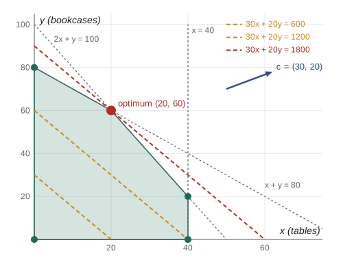
$The feasible pentagon of the shop model in the x y plane, with vertices at (0, 0), (40, 0), (40, 20), (20, 60) and (0, 80). Dashed level lines of 30 x plus 20 y equal 600, 1200 and 1800 run diagonally down to the right; the 1800 line touches the pentagon only at the vertex (20, 60), which is marked optimal. An arrow shows the direction of the gradient (30, 20).$

The shop's feasible region and level lines of the profit. The line $30x + 20y = 1800$ touches the region only at $(20, 60)$, so that vertex is the unique optimum

For the shop, the level lines have slope $-\frac32$, between the slope $-2$ of the carpentry line and the slope $-1$ of the finishing line. Sliding outward, the last contact is the corner where those two lines meet: solving $2x + y = 100$, $x + y = 80$ gives $x = 20$, $y = 60$, with profit $30 \cdot 20 + 20 \cdot 60 = 1800$ dollars a week. At this plan both carpentry and finishing are fully used, while demand for tables is not reached: $s_3 = 20$.

Worked problem

Reading the optimum from slopes

For which table profits $c_1$ (keeping the bookcase profit at 20) does $(20, 60)$ remain optimal?

Show solution

The level lines $c_1x + 20y = z$ have slope $-c_1/20$.
The corner $(20, 60)$ is the last point of contact exactly when this slope lies between the slopes of the two lines through it, $-2$ (carpentry) and $-1$ (finishing).
So we need $-2 \le -c_1/20 \le -1$, that is $20 \le c_1 \le 40$.
At $c_1 = 20$ the level lines are parallel to the finishing line and every point on the edge from $(0, 80)$ to $(20, 60)$ is optimal; at $c_1 = 40$ they are parallel to the carpentry line and the edge from $(20, 60)$ to $(40, 20)$ is optimal.

Answer: The plan stays optimal for table profits from 20 to 40 dollars. Outside this range the optimum jumps to a neighboring vertex. Lesson 7 develops this kind of sensitivity analysis systematically.

The four possible outcomes

The pictures show that a two-variable LP ends in one of four ways. There may be a unique optimum at a vertex, as for the shop. There may be infinitely many optima filling an edge, when the level lines are parallel to an edge that is the last contact, as at $c_1 = 20$ above. The problem may be unbounded: if the shop had no carpentry or finishing limits, profit could increase forever along the ray $y \to \infty$. Or it may be infeasible: adding the requirement $x + y \ge 90$ to the shop model contradicts the finishing limit $x + y \le 80$, and the feasible set is empty.

Observe what does not happen. The optimum is never strictly inside the polygon, because a linear function with nonzero gradient can always be increased by moving in the direction $c$. And if there is an optimum and the polygon has a corner, some corner is optimal, even when a whole edge is. Unboundedness requires an unbounded feasible set but is not implied by it: minimizing $x + y$ over the unbounded quadrant $x, y \ge 0$ has the optimum $(0, 0)$. Lesson 3 proves these facts in any dimension. Unlike general nonlinear programs, an LP whose optimal value is finite always attains it; there is no LP analog of minimizing $e^x$.

Convexity of the feasible set

A set $C$ is convex if whenever $u, w \in C$, the whole segment $\{\lambda u + (1 - \lambda)w : 0 \le \lambda \le 1\}$ lies in $C$. The feasible set of an LP is always convex. Indeed, if $Au \le b$ and $Aw \le b$ and $0 \le \lambda \le 1$, then

\[A(\lambda u + (1 - \lambda)w) = \lambda Au + (1 - \lambda)Aw \le \lambda b + (1 - \lambda)b = b,\]

where the inequality uses $\lambda \ge 0$ and $1 - \lambda \ge 0$. The same argument shows that the set of optimal solutions of an LP is convex: if $u$ and $w$ are optimal with value $z^*$, every point between them is feasible with value $\lambda z^* + (1 - \lambda)z^* = z^*$. This is why multiple optima come as whole edges or faces, never as two isolated points. Lesson 9 shows convexity is the deep reason linear programming is tractable.

Enumerating vertices

In two variables the corners can be found by brute force: every corner is the intersection of two constraint lines, so solve each pair of lines, keep the intersection points that satisfy all the constraints, and evaluate the objective at each. The program does this in exact rational arithmetic using Python's fractions module and Cramer's rule. It reports which two constraints are tight at each vertex and compares three objectives: the shop's profit, a profit with equal margins showing an edge of optima, and a bookcase-heavy profit that moves the optimum to another corner.

Exact vertex enumeration for the shop model with three different objectives

from fractions import Fraction as Fr
from itertools import combinations

# constraints a1 x + a2 y <= b, including the sign constraints -x <= 0, -y <= 0
cons = [((2, 1), 100, "carpentry"), ((1, 1), 80, "finishing"), ((1, 0), 40, "demand"),
        ((-1, 0), 0, "x >= 0"), ((0, -1), 0, "y >= 0")]

def vertices(cons):
    pts = []
    for (a, b, n1), (c, d, n2) in combinations(cons, 2):
        det = a[0] * c[1] - a[1] * c[0]
        if det == 0:
            continue                       # parallel lines never meet in one point
        x = Fr(b * c[1] - a[1] * d, det)   # Cramer's rule
        y = Fr(a[0] * d - b * c[0], det)
        if all(p[0] * x + p[1] * y <= q for p, q, _ in cons):
            if (x, y) not in [v for v, _ in pts]:
                pts.append(((x, y), (n1, n2)))
    return pts

V = vertices(cons)
for obj in [(30, 20), (20, 20), (10, 30)]:
    print(f"objective {obj[0]}x + {obj[1]}y:")
    best = max(obj[0] * x + obj[1] * y for (x, y), _ in V)
    for (x, y), tight in sorted(V):
        z = obj[0] * x + obj[1] * y
        mark = "  <- optimal" if z == best else ""
        print(f"   vertex ({x}, {y})  tight: {tight[0]:9s} + {tight[1]:9s}  value {z}{mark}")
print("pairs of lines examined:", len(list(combinations(cons, 2))), " feasible vertices:", len(V))

Output

objective 30x + 20y:
   vertex (0, 0)  tight: x >= 0    + y >= 0     value 0
   vertex (0, 80)  tight: finishing + x >= 0     value 1600
   vertex (20, 60)  tight: carpentry + finishing  value 1800  <- optimal
   vertex (40, 0)  tight: demand    + y >= 0     value 1200
   vertex (40, 20)  tight: carpentry + demand     value 1600
objective 20x + 20y:
   vertex (0, 0)  tight: x >= 0    + y >= 0     value 0
   vertex (0, 80)  tight: finishing + x >= 0     value 1600  <- optimal
   vertex (20, 60)  tight: carpentry + finishing  value 1600  <- optimal
   vertex (40, 0)  tight: demand    + y >= 0     value 800
   vertex (40, 20)  tight: carpentry + demand     value 1200
objective 10x + 30y:
   vertex (0, 0)  tight: x >= 0    + y >= 0     value 0
   vertex (0, 80)  tight: finishing + x >= 0     value 2400  <- optimal
   vertex (20, 60)  tight: carpentry + finishing  value 2000
   vertex (40, 0)  tight: demand    + y >= 0     value 400
   vertex (40, 20)  tight: carpentry + demand     value 1000
pairs of lines examined: 10  feasible vertices: 5

Of the ten pairs of lines, one pair is parallel ($x = 40$ and $x = 0$) and four intersect outside the feasible region, leaving the five corners of the pentagon. With equal profits of 20 the two endpoints of the finishing edge tie, signaling an edge of optima, and with a bookcase profit of 30 the optimum moves to $(0, 80)$. Brute force is fine here but explodes in higher dimensions: with $m$ constraints in $n$ variables there are up to $\binom{m}{n}$ candidate intersections, and for 50 constraints in 25 variables that is more than $10^{14}$. The simplex method of lesson 4 visits only a short path of vertices, each better than the last.

Common mistakes

MistakeWriting a percentage requirement such as "at least 30 percent protein" as $0.09x_1 + 0.60x_2 \ge 0.30$.
InsteadThe requirement is relative to the total: $0.09x_1 + 0.60x_2 \ge 0.30(x_1 + x_2)$, which is linear after expanding.
MistakeForgetting the nonnegativity constraints.
InsteadWithout $x, y \ge 0$ the shop could make negative tables to free carpentry hours; always state sign restrictions.
MistakeThinking the optimum might lie inside the feasible polygon.
InsteadA nonzero linear objective can always be improved by moving in the direction of its gradient, so optima lie on the boundary.
MistakeConcluding that an unbounded feasible set means an unbounded LP.
InsteadIt depends on the objective: minimizing $x + y$ on $x, y \ge 0$ has the optimum $(0, 0)$.
MistakeTreating two different optimal vertices as the only optimal solutions.
InsteadThe optimal set is convex, so the whole segment between them is optimal.

Summary and key terms

A linear program optimizes a linear objective subject to linear constraints; proportionality and additivity are the modeling assumptions.
Production, blending and transportation are classic LP models; ratio constraints become linear by clearing denominators.
Slack, surplus and split variables convert any LP to standard form: minimize $c^Tx$ subject to $Ax = b$, $x \ge 0$.
In two variables the feasible set is a convex polygon and level lines of the objective slide in the direction of $c$.
An LP has a unique optimum, an edge or face of optima, is unbounded, or is infeasible; finite optimal values are always attained.
The feasible set and the optimal set of an LP are convex.

linear program: An optimization problem with a linear objective and linear equality and inequality constraints.
slack variable: A nonnegative variable that turns a less-than-or-equal constraint into an equation and measures unused capacity.
standard form: Minimize c transpose x subject to Ax = b and x nonnegative.
half-plane: The set of points on one side of a line, including the line.
level line: A set on which the objective takes a constant value.
convex set: A set containing the segment between any two of its points.

Practice problems

Work each problem on paper first, then reveal the answer to check.

Solve the shop model graphically if the finishing hours rise from 80 to 90.
Show answer
The carpentry and finishing lines now meet at $x = 10$, $y = 80$, with profit 1900. Check the slopes: the level lines still lie between the two boundary slopes, so this corner is optimal.
Convert to standard form: maximize $x_1 - x_2$ subject to $x_1 + x_2 \ge 2$, $x_1 - x_2 \le 3$, $x_1 \ge 0$, $x_2$ free.
Show answer
Minimize $-x_1 + x_2^+ - x_2^-$ subject to $x_1 + x_2^+ - x_2^- - s_1 = 2$, $x_1 - x_2^+ + x_2^- + s_2 = 3$, all variables nonnegative.
Sketch the feasible set of $x + y \ge 2$, $x - y \le 1$, $x, y \ge 0$. Is minimizing $x + 2y$ bounded? Is maximizing it?
Show answer
The set is unbounded upward. Minimizing $x + 2y$ is bounded, with optimum at $(1.5, 0.5)$, value 2.5; maximizing is unbounded along $y \to \infty$.
Verify the feed blend answer and find which constraint has slack.
Show answer
$x_1 = 8000/17 \approx 470.6$, $x_2 = 5600/17 \approx 329.4$. Protein is tight; fiber is $0.03x_1 - 0.01x_2 \approx 10.8 > 0$, so fiber has slack.
Show that the set of optimal solutions of an LP is convex.
Show answer
If $u$ and $w$ are feasible with $c^Tu = c^Tw = z^*$, then $\lambda u + (1 - \lambda)w$ is feasible by convexity of the feasible set, and its value is $\lambda z^* + (1 - \lambda)z^* = z^*$.
Formulate: two warehouses with supplies 30 and 40, three stores with demands 20, 25, 25, and costs $c_{ij}$. How many variables and constraints?
Show answer
Six variables $x_{ij} \ge 0$; two supply constraints $\sum_j x_{ij} \le s_i$ and three demand constraints $\sum_i x_{ij} \ge d_j$, plus nonnegativity.