
MATH-372 · Lesson 5 of 12 · 29 min
Degeneracy, cycling and the two-phase method
The simplex method of lesson 4 came with two loose ends. Its termination proof assumed that no basic feasible solution is degenerate, and it needed a starting basic feasible solution, which was obvious only for problems of the form \(Ax \le b\) with \(b \ge 0\). This lesson ties up both. Degenerate vertices, where more constraints are active than necessary, allow pivots that change the basis without moving, and in rare cases the method can loop forever through a cycle of such bases. Bland's smallest-index rule provably prevents this. The two-phase method finds a starting vertex, or proves there is none, by first solving an auxiliary LP that has an obvious starting point. Together these give a complete algorithm that decides every linear program, which in turn underpins the duality theory of lesson 6.
Degenerate vertices
In \(\mathbb{R}^n\) a vertex needs \(n\) linearly independent active constraints. If more than \(n\) are active, the vertex is degenerate. In standard form this shows up as a basic variable equal to zero, and the same point is the basic solution of several different bases. Degeneracy is not an exotic accident. It arises naturally whenever the data have structure: in assignment and transportation problems, for instance, almost every vertex is degenerate, and in models with many redundant capacity constraints, degeneracy is the rule rather than the exception.
Worked problem
A degenerate shop
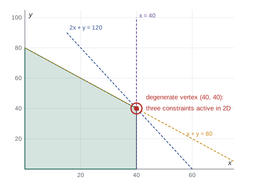
Suppose the shop of lesson 2 has 120 carpentry hours instead of 100. Describe the vertex \((40, 40)\) in standard form and the bases that represent it.
Show solution
- The constraints become \(2x + y + s_1 = 120\), \(x + y + s_2 = 80\), \(x + s_3 = 40\). At \((40, 40)\): \(s_1 = 120 - 120 = 0\), \(s_2 = 0\), \(s_3 = 0\).
- All three slacks vanish, so three inequality constraints are active at a point of \(\mathbb{R}^2\), one more than needed.
- A basis needs three variables. The positive ones, \(x\) and \(y\), must be in it, and the third can be any of \(s_1\), \(s_2\), \(s_3\) that makes the columns independent. All three choices work, giving three bases with the same basic solution, each with one basic variable equal to zero.
- A pivot that swaps one of these zero slacks for another has ratio \(0/u_i = 0\): the basis changes but the point stays at \((40, 40)\).
Answer: The vertex is degenerate and has three representing bases. The simplex method can spend pivots moving among them without changing the objective, which is harmless here but is the mechanism behind cycling.
With degeneracy the argument of lesson 4 breaks down at one point: the step length \(\theta^*\) can be zero, so the cost does not decrease and a basis might be revisited. A degenerate pivot is not wasted, though. Although the point does not move, the basis changes, and after a few degenerate pivots the method usually finds a basis from which an improving edge can actually be followed. The question is whether it is guaranteed to.
Cycling
It is not, with the most natural pivoting rules. Alan Hoffman gave the first example of cycling in 1953, and Martin Beale found a much smaller one in 1955. In Beale's example, written in standard form with slacks \(x_1, x_2, x_3\),
the starting basis \(\{x_1, x_2, x_3\}\) is feasible and highly degenerate, with \(x_1 = x_2 = 0\). Using Dantzig's rule (most negative reduced cost enters) and breaking ties in the ratio test by the smallest index, the method performs six degenerate pivots and returns to the starting basis. It would repeat this cycle forever, never reaching the optimal value \(-\frac54\). Cycling is rare in practice, and early codes simply ignored it, but a theory of linear programming needs an algorithm that provably terminates.
Several remedies are known. The lexicographic rule of Dantzig, Orden and Wolfe (1955) perturbs the right-hand side symbolically so that no vertex is degenerate. Charnes's perturbation method does the same with explicit tiny numbers. The simplest to state and prove is Bland's rule.
Bland's rule
Bland's rule. Among the nonbasic variables with negative reduced cost, the entering variable is the one with the smallest index. Among the rows tied in the minimum ratio test, the leaving variable is the basic variable with the smallest index.
Theorem (Bland, 1977). With Bland's rule, the simplex method cannot cycle. Hence, starting from any basic feasible solution, it terminates after finitely many pivots, either with an optimal basis or with a proof of unboundedness.
Proof. Suppose a cycle of bases occurs. The cost never increases and returns to its starting value, so it is constant: every pivot in the cycle is degenerate, and the basic feasible solution \(x\) itself never changes. Call a variable fickle if it enters (and so also leaves) the basis somewhere in the cycle. Every fickle variable is nonbasic at some point of the cycle, so its value in \(x\) is zero. Let \(t\) be the largest index of a fickle variable.
Some pivot of the cycle has \(x_t\) leaving the basis; call the basis there \(B\) and the entering variable \(x_s\). Then \(s\) is fickle too, so \(s < t\). Some later pivot has \(x_t\) entering; call that basis \(B'\) and its reduced costs \(\bar c'\). Because Bland's rule chose \(t\) at \(B'\), we have \(\bar c'_t < 0\) and \(\bar c'_j \ge 0\) for every \(j < t\).
At \(B\), let \(d\) be the edge direction for the entering \(x_s\): \(d_s = 1\), \(d_{B(i)} = -u_i\) where \(u = B^{-1}A_s\), and \(d_j = 0\) otherwise. Then \(Ad = 0\) and \(c^Td = \bar c_s < 0\). Any reduced cost vector has the form \(\bar c' = c - A^Ty'\) for some \(y'\), so \(\bar c'^Td = c^Td - y'^TAd = c^Td < 0\). We examine the terms of \(\sum_j \bar c'_jd_j < 0\). The term \(j = s\) is \(\bar c'_s \ge 0\), since \(s < t\). The term \(j = t\) is \(\bar c'_t \cdot (-u_t)\), and \(u_t > 0\) because \(x_t\) left the basis at \(B\); this term is positive. All terms with \(j\) outside \(B \cup \{s\}\) vanish. So some \(j \in B\) with \(j \ne t\) has \(\bar c'_jd_j < 0\).
For this \(j\), \(\bar c'_j \ne 0\), so \(x_j\) is nonbasic at \(B'\). It was basic at \(B\), so it leaves somewhere in the cycle and is fickle; hence \(j < t\), and so \(\bar c'_j \ge 0\), in fact \(\bar c'_j > 0\). Then \(d_j = -u_j < 0\), so \(u_j > 0\). Since \(x_j\) is fickle, its value is zero, so its row gives ratio \(x_j/u_j = 0\) in the ratio test at \(B\), tying with the row of \(x_t\), which also had ratio zero because the pivot was degenerate. Bland's tie-breaking would then have chosen the smaller index \(j\) to leave instead of \(t\). This contradiction shows no cycle exists. With no repeated basis and finitely many bases, the method terminates. \(\square\)
Bland's rule is rarely used in production codes because the smallest-index choice ignores the size of the improvement and can be slow, but its proof is the cleanest route to a terminating algorithm, and that is what theory needs.
Finding a first vertex: phase one
For a general standard form problem, minimize \(c^Tx\) subject to \(Ax = b\), \(x \ge 0\), there is no obvious basic feasible solution. First multiply rows by \(-1\) where needed so that \(b \ge 0\). Then introduce one artificial variable \(a_i \ge 0\) for each row and solve the phase one problem
This has the obvious basic feasible solution \(x = 0\), \(a = b\), with the artificials as the basis, and its cost is bounded below by zero, so the simplex method with Bland's rule finds an optimal basis.
Theorem. The original problem is feasible if and only if the phase one optimal value is zero.
Proof. If \(\bar x\) is feasible for the original problem, then \((x, a) = (\bar x, 0)\) is feasible for phase one with cost 0, the smallest possible value, so the optimum is zero. Conversely if the optimum is zero, the optimal \(a\) is zero because \(a \ge 0\) sums to zero, and the optimal \(x\) satisfies \(Ax = b\), \(x \ge 0\). \(\square\)
If the phase one optimum is positive, we stop: the original problem is infeasible, and lesson 6 shows that the final phase one tableau also yields a certificate of infeasibility in the form of a Farkas vector. If it is zero, we have a feasible point, but the final basis may still contain artificial variables at value zero. Each such artificial can be driven out by a degenerate pivot on any nonzero entry of its row in an original column; if the row has no such entry, the row is a linear combination of the others, the corresponding original equation is redundant, and the row can be deleted. After this cleanup we have a basis of original columns, and phase two runs the simplex method on the original objective from there.
An alternative is the big-M method, which adds the artificials to the original objective with a huge penalty \(M\), solving one problem instead of two. It is convenient by hand but numerically awkward, since \(M\) must be large enough without swamping the real costs, and solvers prefer the two-phase approach.
Worked problem
Phase one by hand
Minimize \(x_1 + x_2\) subject to \(x_1 + 2x_2 \ge 4\), \(3x_1 + x_2 \ge 6\), \(x \ge 0\).
Show solution
- Standard form with surplus variables: \(x_1 + 2x_2 - s_1 = 4\), \(3x_1 + x_2 - s_2 = 6\). The origin is not feasible, so add artificials: \(x_1 + 2x_2 - s_1 + a_1 = 4\), \(3x_1 + x_2 - s_2 + a_2 = 6\). Phase one minimizes \(w = a_1 + a_2 = 10 - 4x_1 - 3x_2 + s_1 + s_2\).
- Bland's rule enters \(x_1\), with reduced cost \(-4\). Ratios \(4/1\) and \(6/3 = 2\): \(a_2\) leaves. Now \(x_1 = 2 - \frac13x_2 + \frac13s_2 - \frac13a_2\) and \(w = 2 - \frac53x_2 + s_1 - \frac13s_2 + \frac43a_2\).
- Enter \(x_2\). The \(a_1\) row, \(a_1 = 2 - \frac53x_2 + \cdots\), gives ratio \(\frac65\); the \(x_1\) row gives \(6\). So \(a_1\) leaves, \(x_2 = \frac65\), \(x_1 = \frac85\), and \(w = 0\): the problem is feasible.
- Phase two: in terms of the nonbasic surpluses, \(x_1 = \frac85 - \frac15s_1 + \frac25s_2\) and \(x_2 = \frac65 + \frac35s_1 - \frac15s_2\), so \(x_1 + x_2 = \frac{14}{5} + \frac25s_1 + \frac15s_2\). Both reduced costs are positive.
Answer: The optimum is \(x = (\frac85, \frac65)\) with value \(\frac{14}{5}\). Phase one happened to land on the optimal vertex, so phase two needed no pivots. The reduced costs \(\frac25\) and \(\frac15\) of the surpluses reappear in lesson 6 as the optimal dual solution.
The complete algorithm
Combining phase one, the cleanup of artificials, phase two and Bland's rule gives an algorithm that terminates on every linear program in standard form with one of three outcomes: a proof of infeasibility (positive phase one optimum), an unbounded edge ray, or an optimal basis whose reduced costs are all nonnegative. This is a constructive proof of the fundamental theorem of lesson 3, and more: when an optimum exists, there is an optimal basis \(B\) with \(c_j - c_B^TB^{-1}A_j \ge 0\) for every \(j\). That last statement, the existence of an optimal basis with nonnegative reduced costs, is exactly what lesson 6 needs to prove strong duality.
Cycling and phase one in code
The program implements a minimization tableau with a choice of entering rule. On Beale's example it shows Dantzig's rule cycling through six degenerate bases and Bland's rule escaping the degenerate vertex and reaching the optimum. It then implements the two-phase method and applies it to the feed blend of lesson 2, whose origin is infeasible because at least 800 kg must be produced, and to an infeasible variant.
from fractions import Fraction as Fr

def pivot(T, basis, r, e):
    p = T[r][e]
    T[r] = [v / p for v in T[r]]
    for i in range(len(T)):
        if i != r and T[i][e] != 0:
            f = T[i][e]
            T[i] = [a - f * q for a, q in zip(T[i], T[r])]
    basis[r] = e

def run(T, basis, rule, allowed, limit=50, trace=None):
    """Minimize: last row holds reduced costs and -z. Returns 'optimal', 'unbounded' or 'cycling'."""
    seen = set()
    for k in range(limit):
        key = tuple(sorted(basis))
        if key in seen and trace is not None:
            trace.append(f"basis {key} repeated after {k} pivots")
            return "cycling", k
        seen.add(key)
        red = T[-1][:-1]
        cand = [j for j in allowed if red[j] < 0]
        if not cand:
            return "optimal", k
        e = min(cand) if rule == "bland" else min(cand, key=lambda j: (red[j], j))
        rows = [i for i in range(len(T) - 1) if T[i][e] > 0]
        if not rows:
            return "unbounded", k
        ratio = min(T[i][-1] / T[i][e] for i in rows)
        r = min((i for i in rows if T[i][-1] / T[i][e] == ratio), key=lambda i: basis[i])
        if trace is not None:
            trace.append(f"x{e + 1} enters, x{basis[r] + 1} leaves, step {ratio}, z = {-T[-1][-1]}")
        pivot(T, basis, r, e)
    return "limit", limit

def tableau(A, b, c, basis):
    T = [[Fr(v) for v in row] + [Fr(r)] for row, r in zip(A, b)]
    z = [Fr(v) for v in c] + [Fr(0)]
    for i, j in enumerate(basis):                 # price out the basic columns
        z = [a - z[j] * q for a, q in zip(z, T[i])]
    T.append(z)
    return T

# Beale's 1955 example, variables x1..x7, starting basis {x1, x2, x3}
A = [[1, 0, 0, Fr(1, 4), -8, -1, 9], [0, 1, 0, Fr(1, 2), -12, Fr(-1, 2), 3], [0, 0, 1, 0, 0, 1, 0]]
b = [0, 0, 1]
c = [0, 0, 0, Fr(-3, 4), 20, Fr(-1, 2), 6]
for rule in ("dantzig", "bland"):
    T, basis, tr = tableau(A, b, c, [0, 1, 2]), [0, 1, 2], []
    status, k = run(T, basis, rule, range(7), trace=tr)
    print(f"{rule} rule: {status} after {k} pivots")
    for line in tr:
        print("   ", line)
    if status == "optimal":
        x = [Fr(0)] * 7
        for i, j in enumerate(basis):
            x[j] = T[i][-1]
        print("    x =", [str(v) for v in x], " z =", -T[-1][-1])

# two-phase method for: minimize c^T x, A x = b, x >= 0 (b >= 0)
def two_phase(A, b, c):
    m, n = len(A), len(A[0])
    Aa = [row + [int(i == k) for k in range(m)] for i, row in enumerate(A)]   # add artificials
    T, basis = tableau(Aa, b, [0] * n + [1] * m, list(range(n, n + m))), list(range(n, n + m))
    run(T, basis, "bland", range(n + m))
    if -T[-1][-1] > 0:
        return "infeasible", -T[-1][-1]
    for i, j in enumerate(basis):                 # drive any zero artificial out of the basis
        if j >= n:
            e = next((k for k in range(n) if T[i][k] != 0), None)
            if e is not None:
                pivot(T, basis, i, e)
    T = [row[:n] + [row[-1]] for row in T[:-1]]
    keep = [i for i, j in enumerate(basis) if j < n]  # rows still holding artificials are redundant
    T, basis = [T[i] for i in keep], [basis[i] for i in keep]
    T = tableau([row[:-1] for row in T], [row[-1] for row in T], c, basis)
    status, _ = run(T, basis, "bland", range(n))
    if status != "optimal":
        return status, None
    x = [Fr(0)] * n
    for i, j in enumerate(basis):
        x[j] = T[i][-1]
    return "optimal", (x, -T[-1][-1])

# feed blend: x1 corn, x2 meal, surplus s1, s2 for the >= rows, slack s3 for fibre
A = [[1, 1, -1, 0, 0], [Fr(-21, 100), Fr(30, 100), 0, -1, 0], [Fr(-3, 100), Fr(1, 100), 0, 0, 1]]
status, (x, z) = two_phase(A, [800, 0, 0], [Fr(3, 10), Fr(9, 10), 0, 0, 0])
print(f"feed blend: {status}, corn {x[0]} = {float(x[0]):.2f} kg, meal {x[1]} = {float(x[1]):.2f} kg, cost {float(z):.2f}")
# an infeasible variant: also demand x1 + x2 <= 700
A2 = [row + [0] for row in A] + [[1, 1, 0, 0, 0, 1]]
print("with total at most 700 kg:", two_phase(A2, [800, 0, 0, 700], [Fr(3, 10), Fr(9, 10), 0, 0, 0, 0])[0])dantzig rule: cycling after 6 pivots
x4 enters, x1 leaves, step 0, z = 0
x5 enters, x2 leaves, step 0, z = 0
x6 enters, x4 leaves, step 0, z = 0
x7 enters, x5 leaves, step 0, z = 0
x1 enters, x6 leaves, step 0, z = 0
x2 enters, x7 leaves, step 0, z = 0
basis (0, 1, 2) repeated after 6 pivots
bland rule: optimal after 6 pivots
x4 enters, x1 leaves, step 0, z = 0
x5 enters, x2 leaves, step 0, z = 0
x6 enters, x4 leaves, step 0, z = 0
x1 enters, x5 leaves, step 0, z = 0
x2 enters, x3 leaves, step 1/2, z = 0
x4 enters, x2 leaves, step 1, z = -1/2
x = ['3/4', '0', '0', '1', '0', '1', '0'] z = -5/4
feed blend: optimal, corn 8000/17 = 470.59 kg, meal 5600/17 = 329.41 kg, cost 437.65
with total at most 700 kg: infeasibleUnder Dantzig's rule every one of the six pivots has step 0, and the basis \(\{x_1, x_2, x_3\}\) recurs: a genuine cycle. Bland's rule makes the same first three choices, then deviates at the fourth pivot by entering \(x_1\) (the smallest index) rather than \(x_7\) (the most negative reduced cost), after which it finds a nondegenerate pivot and reaches \(x = (\frac34, 0, 0, 1, 0, 1, 0)\) with cost \(-\frac54\). The two-phase method reproduces the feed blend of lesson 2 exactly, \(\frac{8000}{17}\) kg of corn and \(\frac{5600}{17}\) kg of meal at 437.65 dollars, and correctly reports that no blend of at most 700 kg can meet the 800 kg requirement.
Common mistakes
MistakeConcluding that a pivot with step zero means the LP is optimal.
InsteadA degenerate pivot changes the basis without moving; optimality is decided only by the reduced costs.
MistakeThinking cycling means the LP has no solution.
InsteadCycling is a failure of the pivoting rule, not of the problem; Bland's rule always terminates.
MistakeStarting phase one with a negative right-hand side.
InsteadMultiply such rows by \(-1\) first, so that \(a = b \ge 0\) is feasible.
MistakeStopping after phase one with an artificial variable still basic and calling the basis final.
InsteadPivot zero-valued artificials out on any nonzero original entry, or delete their rows as redundant.
MistakeTreating a positive phase one optimum as unboundedness.
InsteadIt means the original constraints have no solution at all.
Summary and key terms
- A degenerate vertex has more active constraints than the dimension; in standard form some basic variable is zero.
- Degenerate pivots change the basis without moving the point, and with some pivoting rules they can cycle forever (Hoffman 1953, Beale 1955).
- Bland's smallest-index rule provably prevents cycling, so the simplex method always terminates.
- Phase one minimizes the sum of artificial variables; the original LP is feasible exactly when this minimum is zero.
- After phase one, zero artificials are pivoted out or their rows deleted as redundant, and phase two optimizes the true objective.
- The complete method decides every LP: infeasible, unbounded, or optimal with nonnegative reduced costs.
- degenerate vertex
- A vertex where more constraints are active than the dimension of the space.
- degenerate pivot
- A pivot with step length zero, which changes the basis but not the point.
- cycling
- An infinite loop of the simplex method through a repeating sequence of bases.
- Bland's rule
- Choose the smallest eligible index for both the entering and the leaving variable.
- artificial variable
- An auxiliary variable added to each row to create an obvious starting basis.
- phase one
- The auxiliary LP minimizing the sum of artificial variables, used to find a feasible basis.
Practice problems
Work each problem on paper first, then reveal the answer to check.
Is the vertex \((0, 0)\) of \(\{x + y \le 1,\ x - y \le 0,\ x, y \ge 0\}\) degenerate?
Show answer
Yes: \(x \ge 0\), \(y \ge 0\) and \(x - y \le 0\) are all active at the origin, three constraints in \(\mathbb{R}^2\).
Use phase one to show that \(x_1 + x_2 = 1\), \(x_1 + x_2 = 2\), \(x \ge 0\) is infeasible.
Show answer
Phase one minimizes \(a_1 + a_2 = 3 - 2x_1 - 2x_2\). Entering \(x_1\), the first row limits it to 1, giving \(a_1 = 0\), \(a_2 = 1\). The reduced costs are then nonnegative, so the optimum is 1 > 0: infeasible.
Why must every pivot in a cycle be degenerate?
Show answer
Each pivot changes the cost by \(\theta^*\bar c_j \le 0\). Returning to the starting basis returns the cost to its starting value, so every change is zero, which with \(\bar c_j < 0\) forces \(\theta^* = 0\).
In the phase one example, why did the method stop after two pivots?
Show answer
After \(a_1\) left, \(w = a_1 + a_2\) expressed in the nonbasic variables has nonnegative coefficients and value 0, its smallest possible value.
Explain why a row of the final phase one tableau with an artificial basic variable and zeros in every original column means a redundant equation.
Show answer
That row expresses a combination of the original equations in which every original column cancels, so the combination of left sides is identically zero; since the system is feasible, the right sides combine to zero too, and the equation adds no information.
With the big-M method, write the objective for the phase one example with original cost \(x_1 + x_2\).
Show answer
Minimize \(x_1 + x_2 + M(a_1 + a_2)\) subject to the equations with artificials, for a large constant \(M\).
Lesson quiz · 5 questions
Score 60% or more to complete this lesson.
Create a free account to save your progress, take quizzes and earn a certificate.