
GEOM-430 · Lesson 9 of 12 · 20 min
Time-dependent coordinates
For most of the history of surveying, a coordinate was a fixed property of a monument. If a control point's published coordinates changed, it meant the monument had been disturbed or the network readjusted. Modern geodesy has turned that idea around. A coordinate is a value at an epoch, and the published description of a point includes how its coordinates change with time. This lesson explains how such coordinates are modeled, how a surveyor moves them from one epoch to another, and what goes wrong when epochs are ignored.
Trajectory models
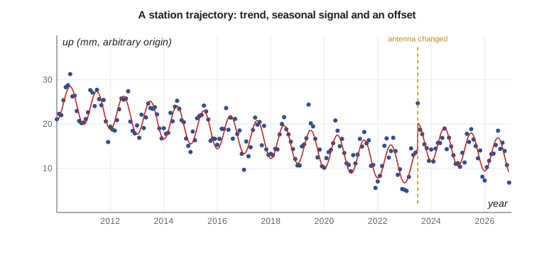
The position of a continuously observed station is a time series. Plotting its daily east, north and up coordinates over several years shows a trend, an annual cycle, occasional jumps and noise. A trajectory model describes these parts with a few parameters.
The terms are the position at the reference epoch t₀, a constant velocity, annual and semi-annual terms, offsets Δ at epochs tⱼ (H is a step function), logarithmic or exponential postseismic decay after earthquakes, and the remaining noise ε. Offsets come from equipment changes, earthquakes, and sometimes unknown causes. Detecting them is one of the most important and most error-prone steps in analyzing a time series; a missed offset biases the velocity, and a false one removes real motion.
Noise in time series
The residuals of a good trajectory model are not white noise. GNSS time series show power-law noise, in which slow, wandering errors are much larger than independent day-to-day scatter would suggest. Its sources include monument instability, unmodeled loading, errors in orbits and in antenna models, and changes in the environment around the antenna. The practical result, mentioned in lesson 3, is that velocity uncertainties computed as if the noise were white are too small by a factor of several, and that offsets of a few millimeters can be hard to distinguish from the noise. Software for time series analysis estimates the noise model with the trajectory so that uncertainties are realistic.
Finding offsets
Offsets come in two kinds. Known offsets have a recorded cause: an antenna or receiver change, a firmware update that changes how the signals are tracked, an earthquake, or work on the monument. Site logs exist so that analysts can find them, and agencies ask station operators to report every change. Unknown offsets show up in the data with no recorded cause, from a tree growing near the antenna, a snow cap on the radome, a change in the processing, or something no one noticed. Statistical tests can find large unknown offsets, but those of a few millimeters in a noisy vertical series often go unnoticed for years.
Comparisons between automatic and manual offset detection, run by the geodetic research community in the 2010s, found that experienced analysts still beat algorithms on difficult series, and that the best results came from combining both. The practical lesson for station operators is simple. Change equipment as rarely as possible, record every change in the site log on the day it happens, and if a change is unavoidable, run the old and new antennas side by side for a while so that the offset can be measured directly.
For CR1, Leah follows that advice when the district asks to replace the original antenna with a newer model able to track all the modern signals. Grant installs the new antenna on a temporary mount a meter away and runs both for six weeks. The difference between the two sets of daily positions, after the known eccentricity is removed, gives the offset that the trajectory model needs, and the site log records the date, the antenna types, their serial numbers and the measured offset. The national agency, which will process CR1's data for years to come, gets a copy the same day, so that the change is never mistaken for motion of the ground.
Moving coordinates between epochs
Because coordinates change, every coordinate must carry its epoch, and transforming a coordinate means moving it in two ways: between frames and between epochs. Mixing up the two is a classic error. A survey observed in 2026 and computed in ITRF2020 gives ITRF2020 coordinates at epoch 2026.84. To compare it with published control at the frame's reference epoch, the surveyor must either move the new coordinates back to the reference epoch or move the control forward, using velocities.
In a global frame, the velocities are dominated by plate motion, so the epoch matters at the level of 15 to 20 mm per year in North America. In a plate-fixed national frame the velocities are small, typically a millimeter or two per year horizontally away from plate boundaries, but GIA, boundary deformation and local motion remain. Agencies therefore publish velocity models for their national frames: grids of velocity covering the country, from which the velocity at any point can be interpolated.
In the United States, NAD83(2011) has an epoch of 2010.00, and the tool HTDP has long been used to move coordinates between epochs with a model of crustal velocity. NATRF2022 has a reference epoch of 2020.00 and an intra-frame velocity model, IFVM, which describes the small motions remaining after the plate's rotation has been removed. The National Geodetic Survey's coordinate conversion and transformation tool, NCAT, will apply both when the new frame is released, and NGS has said the frames will be time-dependent, so that published coordinates will be accompanied by velocities.
An example at CR1
The code models CR1's position in NATRF2022, in a local east, north, up system around its reference-epoch position. The velocity is about 0.4 mm per year east, −0.6 mm per year north and −0.9 mm per year up, an annual vertical cycle of 4 mm, and an offset of 1.5, −0.8 and 6.0 mm when the antenna was changed in mid-2023. It then takes a position observed in November 2026 and brings it back to the reference epoch.
import math
# A station trajectory model: position at epoch t from a reference position, velocity, seasonal terms and an offset.
t0 = 2020.0                          # reference epoch of the frame
X0 = (0.0, 0.0, 0.0)                          # east, north, up at t0 (m, local frame)
V = (0.4, -0.6, -0.9)                            # velocity, mm/yr (east, north, up)
amp_up, phase = 4.0, 0.25          # annual vertical signal, mm and fraction of a year
offset = (2023.5, (1.5, -0.8, 6.0))                   # (epoch, (de, dn, du) mm), e.g. an antenna change
def position(t):
    dt = t - t0
    e, n, u = (X0[i] + V[i] * dt / 1000 for i in range(3))
    u += amp_up / 1000 * math.sin(2 * math.pi * (t - phase))
    if t >= offset[0]:
        e += offset[1][0] / 1000; n += offset[1][1] / 1000; u += offset[1][2] / 1000
    return e, n, u
for t in sorted({t0, 2020.0, 2024.5, 2026.84}):
    e, n, u = position(t)
    print(f"epoch {t:8.2f}: E {e:.4f}  N {n:.4f}  U {u:.4f}")
# Epoch change: survey observed at 2026.84 brought back to the frame epoch, ignoring the seasonal term
obs = position(2026.84)
back = [obs[i] - V[i] * (2026.84 - t0) / 1000 - offset[1][i] / 1000 for i in range(3)]
print("brought to reference epoch:", " ".join(f"{v:.4f}" for v in back))
print(f"horizontal motion since {t0}: {math.hypot(V[0], V[1]) * (2026.84 - t0):.1f} mm")epoch 2020.00: E 0.0000 N 0.0000 U -0.0040 epoch 2024.50: E 0.0033 N -0.0035 U 0.0060 epoch 2026.84: E 0.0042 N -0.0049 U -0.0023 brought to reference epoch: 0.0000 -0.0000 -0.0021 horizontal motion since 2020.0: 4.9 mm
Between 2020.0 and late 2026, the model moves CR1 about 5 mm horizontally and, with the offset and the seasonal term, by a few millimeters vertically. Bringing the 2026 observation back with the velocity and the offset recovers the reference-epoch position, except for 2 mm in height, which is the seasonal term the back-propagation ignored. That residual is a reminder that a single observation at any time of year carries the seasonal signal unless it is modeled.
The same calculation in ITRF2020, with the plate's 17 to 18 mm per year included, would move CR1 by more than 20 cm since 2015. That is why national frames exist, but also why a surveyor taking coordinates from a precise point positioning service, which delivers ITRF at the epoch of observation, must transform them properly before comparing them with national control.
Epochs in practice
Time-dependent coordinates raise practical questions that every firm must answer in its procedures. Which epoch should a project use? Most projects adopt one epoch, often the national frame's reference epoch or a project epoch near the start of construction, and transform all observations to it. Should old coordinates be updated? For control used over many years in a region with significant motion, yes; otherwise surveys of different dates will not fit. What should be written on plans and in data files? The frame, its version, and the epoch, every time.
| Situation | What to record | Typical action |
|---|---|---|
| GNSS processed with a PPP service | ITRF realization and epoch of observation | Transform to the national frame at the project epoch |
| RTK from a provincial or state network | The network's frame, version and epoch | Check against published control at the same epoch |
| Old control from a previous adjustment | Frame, version, epoch, adjustment name | Transform or re-observe before combining |
| Monitoring over years | Epoch of every measurement | Analyze as time series with velocities |
Many errors in practice come from software that silently assumes an epoch. A GIS package may treat two frames as identical, or a field controller may label coordinates with a frame but not an epoch. At the centimeter level that rarely matters in a plate-fixed frame over a few years, but it matters when mixing global and national frames, when comparing surveys decades apart, or in regions of active deformation. The rule Ruth applies at Coulee Geomatics is that a coordinate without a frame and an epoch is a coordinate that cannot be checked.
Worked problem
How far has a point moved since the frame epoch?
A point in a plate-fixed frame has a residual velocity of 1.2 mm per year east and 2.1 mm per year down. How much has it moved between epoch 2010.0 and epoch 2027.0?
Show solution
- \[\Delta t = 17.0\ \text{yr}\]
- \[\Delta e = 1.2 \times 17 = 20\ \text{mm}, \quad \Delta u = -2.1 \times 17 = -36\ \text{mm}\]
Answer: About 20 mm east and 36 mm down: enough to matter for precise heights.
Deformation models
Where deformation is not smooth, a velocity grid is not enough. Earthquakes create offsets that vary across a region, and postseismic motion follows its own course. Countries on active margins publish deformation models that combine a secular velocity field with patches for each significant earthquake, each with its own time function. New Zealand's national deformation model, built into its frame since 2000 and updated after each major earthquake, is the best-known example. Canada and the United States have not needed one at that scale away from the west coast and Alaska, but a great Cascadia earthquake would require one, and agencies plan for it.
Glacial isostatic adjustment is the other large, slowly varying signal. Its vertical rate is up to a centimeter per year around Hudson Bay, so heights and ellipsoidal heights there change by decimeters over a few decades. Velocity models in both countries include it, and lesson 11 shows that heights must be treated as time-dependent too.
Coulee Geomatics: the district's records
Leah writes a two-page procedure for the district's data managers. It asks that every coordinate in the district's GIS carry the frame, version and epoch, and that GNSS surveys from contractors be accepted only with those labels. It explains, with CR1 as an example, why the same monument has different coordinates in different frames and epochs and how to convert them with the national tools. It sets a project epoch for the headworks work and asks contractors to deliver coordinates at that epoch. And it recommends that the district's own control points be re-observed every five years, with the results compared as a time series rather than replaced.
Common mistakes
MistakeRecording a GNSS coordinate without its epoch.
InsteadAlways record the frame, its version and the epoch.
MistakeTreating a frame transformation as an epoch transformation.
InsteadThey are different steps; apply both when needed.
MistakeFitting a velocity without modeling known offsets.
InsteadModel equipment changes and earthquakes as offsets in the trajectory.
MistakeUsing white-noise velocity uncertainties.
InsteadEstimate a realistic noise model; GNSS noise is correlated in time.
Summary and key terms
- A coordinate is a value at an epoch; the published description includes velocity.
- Trajectory models combine position, velocity, seasonal terms, offsets and postseismic decay.
- GNSS time series contain correlated noise, so realistic uncertainties are larger than formal ones.
- National frames have reference epochs and velocity models for moving coordinates in time.
- Every coordinate must be labeled with frame, version and epoch.
- Active regions need deformation models with earthquake patches.
- Trajectory model
- A model of a station's position as a function of time.
- Reference epoch
- The epoch at which a frame's coordinates are published.
- Velocity grid
- A grid of velocities from which a point's velocity can be interpolated.
- Offset
- A sudden change in a station's position, from equipment changes or earthquakes.
- Power-law noise
- Noise whose power increases at low frequencies, as in GNSS time series.
- Deformation model
- A model combining velocities and earthquake effects for a region.
Practice problems
Work each problem on paper first, then reveal the answer to check.
A station has velocity −14 mm per year east in ITRF. Its coordinates at epoch 2015.0 are used for a survey at 2027.0. What is the east error?
Show answer
−14 × 12 = −168 mm.
Why can a missed offset bias a velocity?
Show answer
The trend fitted across the jump absorbs part of it.
What should a coordinate label include?
Show answer
The frame, its version and the epoch.
Why is a single GNSS observation affected by the season?
Show answer
Seasonal loading moves the station by a few millimeters, especially vertically.
What do deformation models add to velocity grids?
Show answer
Offsets and postseismic motion from individual earthquakes.
Lesson quiz · 5 questions
Score 60% or more to complete this lesson.
Create a free account to save your progress, take quizzes and earn a certificate.