
GEOM-350 · Lesson 7 of 12 · 18 min
Classification
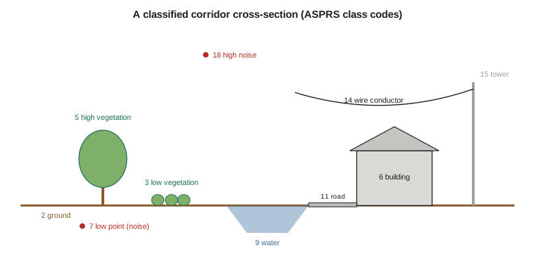
Ground filtering divides the corridor's points into two groups. The district needs more: the vegetation along the canal banks, which affects seepage and maintenance access; the buildings at the headworks yard and the farmsteads, for the floodplain inventory; the power line conductors, towers and poles, for clearance checks; the canal water surface; the road; the bridges. Assigning each point a class is called classification, or semantic segmentation in the computer vision literature. This lesson describes the standard classes, the features that make classification possible, and the rule-based and machine learning methods that use them.
Point cloud formats and classes
Lidar data are exchanged mostly in the LAS format published by ASPRS, the American Society for Photogrammetry and Remote Sensing, now at version 1.4, or in LAZ, a lossless compressed form of LAS that is several times smaller. A LAS file has a header describing the coordinate reference system, extent, scale and offset; optional variable-length records with metadata such as the coordinate system's well-known text; and the point records. Each point record stores the coordinates as scaled integers, the intensity, the return number and number of returns, the scan angle, the GPS time, the classification code, flags such as withheld and overlap, and, in some point formats, color, near-infrared values or a pointer to the waveform. Terrestrial scans are often exchanged in E57, an ASTM standard format that can also store each scan's position and images.
The classification codes are standardized. LAS 1.4 defines codes 0 to 22 for common classes and leaves the rest for users and domain profiles:
| Code | Class | Code | Class |
|---|---|---|---|
| 0 | Created, never classified | 11 | Road surface |
| 1 | Unclassified | 13 | Wire guard (shield) |
| 2 | Ground | 14 | Wire conductor (phase) |
| 3 | Low vegetation | 15 | Transmission tower |
| 4 | Medium vegetation | 16 | Wire-structure connector (insulator) |
| 5 | High vegetation | 17 | Bridge deck |
| 6 | Building | 18 | High noise |
| 7 | Low point (noise) | 19 | Overhead structure |
| 9 | Water | 20 | Ignored ground (for example near-vertical surfaces) |
| 10 | Rail | 21 | Snow |
| 22 | Temporal exclusion |
The USGS Lidar Base Specification requires a minimum classification (unclassified, ground, low and high noise, water, bridge deck, ignored ground and snow where present, and the withheld and overlap flags) and allows more. The project's specification asks for codes 1, 2, 3, 5, 6, 7, 9, 14, 15, 17 and 18, plus a user class 64 for the canal's concrete-lined sections. Specifications also define accuracy for classification, such as no more than 2 percent of points misclassified in the ground class, and may require that vegetation height classes be defined by height above ground: for example, low vegetation from 0.15 to 2 m, high vegetation above 5 m.
Features for classification
Classification relies on features computed for each point from the point itself and its neighborhood. Some come directly from the data: height above the ground surface (HAG, computed once ground is classified), intensity, return number and number of returns, and color where cameras were used. A first return that is also the only return is usually a hard surface; a first of several returns is usually vegetation or an edge.
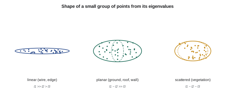
Geometric features describe the local shape. For each point, the covariance matrix of the coordinates of its neighbors is computed and its eigenvalues \(\lambda_1 \ge \lambda_2 \ge \lambda_3\) found. Their relative sizes describe the shape of the neighborhood:
Linearity \(L\) is high for wires and edges, where points spread along one direction; planarity \(P\) is high for ground, roofs and walls; scattering \(S\) is high for vegetation, where points spread in all directions. The eigenvector of the smallest eigenvalue is the local normal, and its vertical component distinguishes horizontal surfaces from walls; verticality \(1 - |n_z|\) is near zero for ground and roofs and near one for walls. Other features include the local point density, the height range within a vertical column, roughness, and the distribution of returns in the column. Because a single neighborhood size cannot suit wires, roofs and trees alike, methods often compute features at several scales.
import math, random
random.seed(3)
def eig3(C):
    """Eigenvalues and vectors of a symmetric 3x3 matrix (cyclic Jacobi), largest first."""
    A = [r[:] for r in C]; V = [[float(i == j) for j in range(3)] for i in range(3)]
    for _ in range(20):
        for p, q in ((0, 1), (0, 2), (1, 2)):
            if abs(A[p][q]) < 1e-14: continue
            th = 0.5 * math.atan2(2 * A[p][q], A[q][q] - A[p][p]); c, s = math.cos(th), math.sin(th)
            for k in range(3):
                A[k][p], A[k][q] = c*A[k][p] - s*A[k][q], s*A[k][p] + c*A[k][q]
            for k in range(3):
                A[p][k], A[q][k] = c*A[p][k] - s*A[q][k], s*A[p][k] + c*A[q][k]
            for k in range(3):
                V[k][p], V[k][q] = c*V[k][p] - s*V[k][q], s*V[k][p] + c*V[k][q]
    order = sorted(range(3), key=lambda i: -A[i][i])
    return [A[i][i] for i in order], [[V[k][i] for k in range(3)] for i in order]

def features(nbhd):
    m = [sum(p[i] for p in nbhd) / len(nbhd) for i in range(3)]
    C = [[sum((p[i] - m[i]) * (p[j] - m[j]) for p in nbhd) / len(nbhd) for j in range(3)] for i in range(3)]
    (l1, l2, l3), vec = eig3(C)
    l1, l2, l3 = (max(x, 1e-12) for x in (l1, l2, l3))
    n = vec[2]
    return {'linearity': (l1 - l2) / l1, 'planarity': (l2 - l3) / l1, 'scatter': l3 / l1,
            'verticality': 1 - abs(n[2])}

# Synthetic local point groups (25 points each) for five kinds of object
def make(kind):
    P = []
    for _ in range(25):
        u, v = random.uniform(-1, 1), random.uniform(-1, 1)
        if kind == 'ground':   P.append([u, v, 0.02 * u + random.gauss(0, 0.01)])
        if kind == 'roof':     P.append([u, v, 0.35 * u + random.gauss(0, 0.01)])
        if kind == 'wall':     P.append([u, random.gauss(0, 0.01), v])
        if kind == 'wire':     P.append([2 * u, random.gauss(0, 0.02), random.gauss(0, 0.02)])
        if kind == 'tree':     P.append([u, v, random.uniform(-1, 1)])
    return P
for kind in ('ground', 'roof', 'wall', 'wire', 'tree'):
    f = features(make(kind))
    print(f"{kind:7s} " + "  ".join(f"{k} {v:.2f}" for k, v in f.items()))

# A rule-based classifier using features and height above ground (HAG)
def classify(f, hag):
    if f['linearity'] > 0.8 and hag > 3: return 'wire'
    if f['scatter'] > 0.15: return 'vegetation'
    if f['verticality'] > 0.7: return 'building' if hag > 0.5 else 'ground'
    if f['planarity'] > 0.5: return 'ground' if hag < 0.3 else 'building'
    return 'unclassified'
cases = [('ground', 0.0, 'ground'), ('roof', 6.0, 'building'), ('wall', 3.0, 'building'), ('wire', 9.0, 'wire'), ('tree', 5.0, 'vegetation')]
labels = ['ground', 'building', 'wire', 'vegetation', 'unclassified']
conf = {(a, b): 0 for a in labels for b in labels}
for _ in range(40):
    for kind, hag, true in cases:
        conf[(true, classify(features(make(kind)), hag + random.gauss(0, 0.5)))] += 1
print("\nconfusion matrix (rows = truth, columns = predicted)")
print(" " * 12 + "".join(f"{l[:8]:>10s}" for l in labels))
for a in labels[:4]:
    print(f"{a:12s}" + "".join(f"{conf[(a, b)]:10d}" for b in labels))
ok = sum(conf[(a, a)] for a in labels); tot = sum(conf.values())
print(f"overall accuracy {ok / tot:.1%}")ground linearity 0.40 planarity 0.60 scatter 0.00 verticality 0.00
roof linearity 0.39 planarity 0.61 scatter 0.00 verticality 0.06
wall linearity 0.12 planarity 0.88 scatter 0.00 verticality 1.00
wire linearity 1.00 planarity 0.00 scatter 0.00 verticality 0.88
tree linearity 0.30 planarity 0.15 scatter 0.56 verticality 0.20
confusion matrix (rows = truth, columns = predicted)
ground building wire vegetati unclassi
ground 26 9 0 0 5
building 0 73 0 0 7
wire 0 0 40 0 0
vegetation 0 0 0 40 0
overall accuracy 89.5%The features separate the five shapes clearly. Ground and roof are planar (planarity about 0.6, scattering near zero) but the roof's normal is tilted; the wall is planar and vertical (verticality 1.00); the wire is almost perfectly linear (1.00); the tree has high scattering (0.56). The simple rules, with height above ground perturbed by half a meter of noise, classify wires and vegetation perfectly and buildings mostly correctly, but they call some ground points building and leave a few unclassified, for an overall accuracy of 89.5 percent. The errors come from a weakness of the rules: they compare height above ground with a fixed 0.3 m threshold, so a noisy height estimate tips planar ground into the building class. Real classifiers combine many more features, tune thresholds from training data, and look at larger context.
Rule-based and object-based classification
Traditional production classification is rule-based: a sequence of algorithms, each tuned by an analyst, applied in order. After ground filtering, points within 0.15 m of the ground might be called ground, points between 0.15 and 2 m low vegetation, and so on by height; building detection then looks for planar patches above a minimum area with sharp height jumps at their edges; wire detection looks for linear features between towers; and the remainder stays as vegetation or unclassified. Analysts then review and edit by hand, tile by tile, often spending more time on editing than on automatic processing. Object-based methods first segment the cloud into objects, such as roof planes, tree crowns or poles, and then classify whole objects using shape, size and context, which reduces the speckled errors that point-by-point methods produce.
Machine learning
Machine learning classifiers learn the relation between features and classes from examples. Random forests and gradient-boosted trees trained on hand-crafted features like those above have been used in production for over a decade; they are fast, need modest training data and their decisions can be inspected through feature importance. Deep learning networks that operate directly on points, on voxels or on graphs of neighboring points learn their own features from large labeled data sets and now achieve the best accuracy on benchmarks for urban and natural scenes, at the cost of large training sets, graphics processors and less transparent decisions. Pre-trained models from vendors and research groups are increasingly available, but they perform best on data like their training data; a model trained on dense urban mobile scans will not perform well on sparse prairie airborne data without retraining.
Whatever the method, training and test data must be separate and representative. Theo labels 24 sample tiles by hand, chosen across the corridor's land cover types, trains on 16 and tests on 8. Labeling is tedious and its own errors limit the accuracy any classifier can show, so two people label the test tiles independently and resolve disagreements.
Measuring classification accuracy
The confusion matrix, introduced in GEOM-320 for images, tabulates true classes against predicted classes for a sample of points. From it come the overall accuracy, the producer's accuracy for each class (the fraction of true members correctly found) and the user's accuracy (the fraction of points given the class that truly belong to it), and summary measures such as the F1 score and the intersection over union used in deep learning papers. Because classes are very unequal in size, with ground and vegetation making up most points and wires a tiny fraction, overall accuracy can look excellent while a small class is badly classified. The district's power line clearance check depends entirely on the wire class, so Leah reports its accuracy separately.
Points can be counted, but area or object accuracy often matters more. A building class that is 95 percent correct by points may still miss small sheds entirely, and a ground class that is 99 percent correct may have its errors concentrated on the canal banks where the engineers need it most. Leah's quality control therefore combines statistics with visual review of profiles across every critical feature.
Using classified data
Classified data feed most products. The bare-earth elevation model uses ground (and, under the 2025 USGS rules and similar practice, sometimes ignored ground and snow treated as specified); a surface model uses first returns or the highest point per cell; a canopy height model subtracts the bare earth from the surface model; building footprints are extracted from the building class; and power line analysis uses wires, towers and vegetation together. Each product inherits the classification's errors, so its metadata should state which classes and returns were used.
Common mistakes
MistakeJudging a classification by overall accuracy alone.
InsteadReport per-class producer's and user's accuracy, especially for small critical classes.
MistakeApplying a pre-trained deep learning model to very different data without testing.
InsteadTest on local labeled samples and retrain if needed.
MistakeTesting a classifier on the tiles used to train it.
InsteadKeep independent test data representative of the whole project.
MistakeAssuming class codes mean the same in every data set.
InsteadCheck the specification and LAS version; reserved and user codes vary.
Summary and key terms
- LAS 1.4 (and compressed LAZ) is the standard format for lidar, with standardized class codes 0 to 22; E57 is common for terrestrial scans.
- Classification uses height above ground, intensity, returns, color and geometric features from neighborhood eigenvalues.
- Linearity, planarity, scattering and verticality distinguish wires, surfaces, vegetation and walls.
- Production classification combines rules, object-based methods, machine learning and manual editing.
- Confusion matrices with per-class accuracy, and visual review of critical features, measure the result.
- Products inherit classification errors; metadata should state the classes used.
- LAS
- The ASPRS binary format for lidar point clouds, with standard fields and classification codes.
- LAZ
- A lossless compressed form of LAS.
- Classification
- Assigning each point a class such as ground, vegetation, building or wire.
- Height above ground
- A point's elevation minus the bare-earth surface beneath it.
- Linearity, planarity, scattering
- Shape features computed from the eigenvalues of a neighborhood's covariance.
- Random forest
- A machine learning classifier made of many decision trees voting together.
- Producer's accuracy
- The fraction of true members of a class that were correctly classified.
- User's accuracy
- The fraction of points assigned a class that truly belong to it.
Practice problems
Work each problem on paper first, then reveal the answer to check.
A point is the first of three returns. Is it more likely ground or vegetation?
Show answer
Vegetation (or an edge); ground points are usually last or only returns.
The eigenvalues of a neighborhood are 0.40, 0.38 and 0.01. What shape is it?
Show answer
Planar (P = 0.93).
Why might a classifier with 98 percent overall accuracy still fail a power line clearance check?
Show answer
The wire class is a tiny fraction of points; its own accuracy may be poor.
Which LAS class code is used for bridge decks?
Show answer
17.
What is a canopy height model?
Show answer
The surface model minus the bare-earth model, giving vegetation height.
Lesson quiz · 5 questions
Score 60% or more to complete this lesson.
Create a free account to save your progress, take quizzes and earn a certificate.