
GEOM-350 · Lesson 6 of 12 · 20 min
Point cloud filtering
The airborne survey arrived as 4.1 billion points in 320 tiles. Before anyone could compute a bare-earth surface, Theo had to clean it. Raw point clouds contain points that belong to nothing: birds, dust, reflections from the canal's surface, returns from below the ground caused by multipath, and noise at the edges of objects. They also contain far more points than some products need. And the most valuable product, the ground surface, has to be separated from the vegetation, buildings and structures above it. This lesson covers the filtering steps that remove noise, reduce data and find the ground.
Kinds of unwanted points
Noise points fall into recognizable kinds. High noise lies well above the real surface: birds, insects, smoke, dust, fog and rain, and spurious returns from atmospheric particles near the aircraft. Low noise lies below the real surface: multipath returns from light that bounced off one surface to another before returning, so that the measured range is too long, and some returns from water and glass. Edge noise, the mixed pixels of lesson 1, forms fringes of points between objects and their backgrounds. Terrestrial scans add their own kinds: ghost points from reflections in windows and polished metal, people and vehicles that moved through the scene, and the tripod and operator near the scanner. Each kind calls for a different filter, and no single filter catches them all.
Filtering decisions are recorded rather than made destructively. In point cloud formats each point carries a classification code (lesson 7), and the usual practice is to classify noise as low noise or high noise rather than delete it, so that a later reviewer can see what was removed and why. Deleted points cannot be recovered; classified points can be reinstated if a filter proves too aggressive.
Statistical and radius outlier removal
Isolated points can be found by looking at their neighborhoods. In statistical outlier removal, the mean distance from each point to its \(k\) nearest neighbors is computed; across the cloud these mean distances have an average \(\mu\) and a standard deviation \(\sigma\), and points whose mean distance exceeds \(\mu + m\sigma\), for a chosen multiplier \(m\), are flagged as outliers. In radius outlier removal, points with fewer than a given number of neighbors within a given radius are flagged. Both work well for birds, dust and isolated low points, and both fail where noise comes in clusters, such as a flock of birds or a patch of fog, or where real features are sparse, such as a thin wire, which can be wrongly removed. The parameters must suit the data's density: a radius right for a terrestrial scan at 5 mm spacing is meaningless for airborne data at 0.2 m.
Elevation-based filters add a simple but effective test. Points more than a set height above or below a coarse surface computed from the data, or a published elevation model, are flagged: for example anything more than 60 m above the ground in a corridor with no tall structures, or more than 2 m below the lowest local ground. Such absolute limits catch gross blunders that statistical filters, tuned to local behavior, may miss.
Reducing the data: thinning and voxel grids
Many tasks do not need every point. A bare-earth surface on a 0.5 m grid needs a few points per cell, not a hundred; a registration needs well-distributed points, not all of them; and a web viewer needs a level of detail suited to the screen. Thinning reduces data in controlled ways. Random thinning keeps a fraction of points; spatial thinning keeps one point per cell of a regular grid or one point per voxel, a small cube of space. Which point is kept matters: the point nearest the cell's center preserves the shape fairly; the lowest point in each cell favors the ground and is a common first step in ground filtering; the highest favors canopy and roofs. Thinning should be done for a stated purpose and recorded, and the original data kept.
Ground filtering
Separating ground from non-ground points is the most important filtering task in airborne lidar, because the bare-earth elevation model drives drainage design, flood mapping, earthworks and most engineering uses. It is also the hardest, because the ground's appearance varies: flat fields, steep coulee banks, canal prisms with sharp breaks, roads on fill, ditches, and low vegetation that sits just above the ground. Dozens of ground filtering algorithms have been published. Most fall into a few families.
Morphological filters use the operations of mathematical morphology on a grid of lowest elevations. An opening, an erosion (taking the minimum in a moving window) followed by a dilation (taking the maximum), removes objects narrower than the window while preserving terrain broader than it. Points that rise above the opened surface by more than a threshold are classed as non-ground. A single window size cannot both remove large buildings and preserve small hills, so progressive morphological filters, such as the one published by Zhang and others in 2003, use a series of growing windows with growing height thresholds: small windows remove shrubs and cars, large ones remove buildings, and the thresholds grow to allow for terrain slope.
Slope-based filters classify a point as ground if the slope from it to its neighboring ground points does not exceed a maximum expected terrain slope. Surface-based filters iteratively build a surface, such as a triangulated irregular network (TIN), from seed ground points, and add points that lie close enough to the surface, by distance and angle, to be ground. Progressive TIN densification, widely used in commercial software, works this way. Cloth simulation filtering turns the cloud upside down and drops a simulated cloth onto it; the cloth settles on the inverted ground and points near the cloth are ground. Machine learning classifiers (lesson 7) are increasingly used as well, often after a conventional filter.
import math, random
random.seed(11)
Z0 = 1010.0
# A 120 m airborne profile across the canal: ground, a berm, shrubs, a power pole and noise
pts = []
for i in range(600):
    x = i * 0.2
    g = Z0 + 0.012 * x + (1.6 if 40 < x < 52 else 0.0) - (2.1 if 70 < x < 78 else 0.0)   # berm and canal
    z = g + random.gauss(0, 0.03)
    if 20 < x < 32 and random.random() < 0.6: z = g + random.uniform(0.3, 2.5)          # shrubs
    if 95 < x < 95.6: z = g + random.uniform(0, 11.0)                                    # pole
    pts.append((x, z, g))
pts += [(37.3, Z0 + 61.2, None), (88.1, Z0 - 14.6, None)]                                # a bird and a multipath low point
print(f"{len(pts)} points")

# 1. Statistical outlier removal: mean distance to the k nearest points
k = 6
def knn_mean(p):
    d = sorted(math.dist(p[:2], q[:2]) for q in pts if q is not p)[:k]
    return sum(d) / k
md = [knn_mean(p) for p in pts]
mu = sum(md) / len(md); sd = math.sqrt(sum((m - mu) ** 2 for m in md) / len(md))
keep = [p for p, m in zip(pts, md) if m < mu + 3 * sd]
print(f"outlier removal (k={k}, 3 sigma): removed {len(pts) - len(keep)} points")

# 2. Thinning to one point per 0.5 m cell (lowest point kept, a common choice before ground filtering)
cells = {}
for p in keep:
    c = int(p[0] // 0.5)
    if c not in cells or p[1] < cells[c][1]: cells[c] = p
thin = [cells[c] for c in sorted(cells)]
print(f"thinned to {len(thin)} lowest points in 0.5 m cells")

# 3. Progressive morphological filter (after Zhang et al. 2003), on the profile
def opening(z, w):
    n = len(z); h = w // 2
    ero = [min(z[max(0, i - h):i + h + 1]) for i in range(n)]
    return [max(ero[max(0, i - h):i + h + 1]) for i in range(n)]
z = [p[1] for p in thin]; ground = [True] * len(z)
surf = z[:]
for w, dh in ((3, 0.25), (7, 0.40), (15, 0.60), (31, 0.90)):     # window in cells, height threshold
    op = opening(surf, w)
    for i in range(len(z)):
        if z[i] - op[i] > dh: ground[i] = False
    surf = op
truth = [p[2] is not None and abs(p[1] - p[2]) < 0.15 for p in thin]
tp = sum(g and t for g, t in zip(ground, truth)); fp = sum(g and not t for g, t in zip(ground, truth))
fn = sum((not g) and t for g, t in zip(ground, truth))
print(f"ground points kept {sum(ground)}: correct {tp}, wrongly called ground {fp}, ground missed {fn}")
miss = [round(p[0], 1) for p, g, t in zip(thin, ground, truth) if t and not g]
print("missed ground near x =", miss[:8], "..." if len(miss) > 8 else "")602 points outlier removal (k=6, 3 sigma): removed 3 points thinned to 240 lowest points in 0.5 m cells ground points kept 212: correct 212, wrongly called ground 0, ground missed 23 missed ground near x = [40.6, 41.4, 41.8, 42.0, 42.8, 43.2, 43.8, 44.4] ...
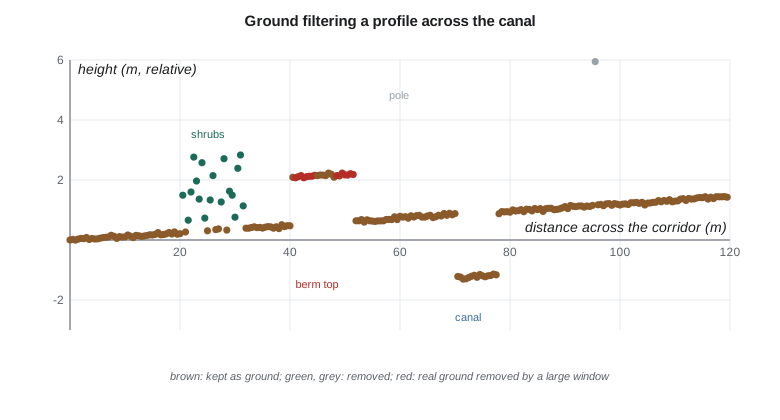
The outlier filter removes the bird 61 m above the ground, the multipath point 15 m below it and the top of the power pole. Thinning keeps the lowest point in each 0.5 m cell, 240 points. The progressive morphological filter then keeps 212 points as ground with no false ground at all, removing the shrubs and the pole, but it also discards 23 real ground points, almost all on the top of the berm between 40 and 52 m. The berm is 1.6 m (5.2 ft) high and 12 m wide; once the window grows past its width, the opening cuts it down and its top rises above the height threshold. This is the classic failure of ground filters at sharp terrain features: berms, road embankments, canal dikes and coulee edges. For the project's canal it is the worst possible place to lose the ground, so Theo runs the filter with a smaller maximum window along the canal and edits the remaining errors by hand against breaklines.
Two kinds of error, and the trade-off between them
Ground filters make two kinds of mistake. Type I errors reject real ground points, as on the berm: the terrain is smoothed, features disappear and sharp edges are rounded. Type II errors accept non-ground points as ground: low vegetation, parked vehicles or parts of structures become bumps in the bare earth. Tightening the parameters reduces one kind and increases the other. Which matters more depends on the use. For flood mapping, losing a berm (a type I error) can change where water goes, while a few shrubs left in (type II) matter little; for volume calculations both matter. Good practice tunes the filter on representative areas, measures both kinds of error against manually classified samples, and documents the settings.
| Terrain or cover | Typical difficulty | Usual remedy |
|---|---|---|
| Steep slopes and coulee banks | Ground on slopes rejected as non-ground | Larger slope tolerance; slope-adaptive thresholds |
| Berms and road embankments | Tops removed by large windows | Smaller windows; breaklines; manual editing |
| Low dense vegetation (crops, grass, shrubs) | Few pulses reach the ground; blended returns sit high | Leaf-off flights; accept a known bias; field checks |
| Bridges and culverts | Decks classed as ground, blocking flow paths | Classify bridge decks separately; hydro-flattening and breaklines |
| Water surfaces | Few returns, noisy points | Classify as water; flatten using breaklines |
| Low buildings and sheds | Small roofs accepted as ground | Building-specific rules; manual review |
Breaklines and hydro-flattening
Bare-earth models used for hydraulics must represent water surfaces and drainage paths correctly. Lidar returns from water are sparse and noisy, and a surface interpolated through them shows false bumps and pits on lakes and rivers. Breaklines are three-dimensional lines along the edges of water bodies, roads, dykes and other sharp features, digitized from the point cloud and imagery and used to constrain the surface so that edges are crisp and water surfaces are flat. Hydro-flattening sets each lake to a single elevation and each river to a smoothly descending surface, bank to bank. Hydro-enforcement goes further, cutting through bridges and culverts so that the model lets water flow where it really does, which is needed for drainage analysis but makes the model unsuitable for other purposes such as road design.
The USGS Lidar Base Specification asks for hydro-flattened bare-earth models with breaklines for water bodies and streams wider than set thresholds, and the county's floodplain program has its own requirements. Theo delivers two bare-earth models: a hydro-flattened one for general use and a hydro-enforced one, with the canal's culverts and the coulee crossings cut through, for the project's drainage modeling. Each is labeled clearly so that nobody designs a road on the enforced one.
Filtering terrestrial and mobile scans
Terrestrial and mobile data need different filters. Moving objects, such as people, vehicles and swaying branches, are removed by comparing overlapping scans: a point present in one scan but seen through in another, where the beam passed through that space to a farther surface, belongs to something that moved. Reflections in glass and water create mirrored copies of real objects, which are recognized by their position behind a reflecting surface and removed. Mixed pixels at edges are removed by thresholds on the angle between the beam and the local surface, or by comparing ranges along a scan line. For the headworks scans, Theo also removes the points on the tripod and the scanner's own shadow, and points beyond 60 m, which add noise without adding information at the spacing needed.
Common mistakes
MistakeDeleting noise points outright.
InsteadClassify them as noise so the decision can be reviewed and reversed.
MistakeUsing the same filter parameters for terrestrial and airborne data.
InsteadParameters depend on density, platform and terrain.
MistakeAssuming the ground filter is right because it runs without error.
InsteadCheck type I and type II errors on sample areas, especially at berms and steep slopes.
MistakeUsing a hydro-enforced model for road design.
InsteadEnforced models cut through embankments; keep a hydro-flattened model for general use.
Summary and key terms
- Raw clouds contain high noise, low noise, edge noise, reflections and moving objects, each needing its own filter.
- Statistical and radius outlier removal flag isolated points; elevation limits catch gross blunders.
- Thinning by grid or voxel reduces data for a stated purpose; which point is kept matters.
- Ground filters (morphological, slope-based, surface-based, cloth simulation, machine learning) separate ground from non-ground.
- Filters trade type I errors (ground rejected) against type II errors (non-ground accepted); berms and steep slopes are hardest.
- Breaklines, hydro-flattening and hydro-enforcement make bare-earth models fit for hydraulics.
- Outlier
- A point far from its neighbors, usually noise.
- Statistical outlier removal
- Flagging points whose mean distance to neighbors is unusually large.
- Voxel
- A small cube of space used to organize or thin a point cloud.
- Ground filter
- An algorithm that separates ground points from points on vegetation and structures.
- Morphological opening
- Erosion followed by dilation, removing objects narrower than the window.
- Breakline
- A three-dimensional line along a sharp terrain feature or water edge that constrains a surface model.
- Hydro-flattening
- Making water surfaces flat and consistent in a bare-earth model.
- Hydro-enforcement
- Modifying a bare-earth model so that water flows through culverts and under bridges.
Practice problems
Work each problem on paper first, then reveal the answer to check.
Why is the lowest point in a cell often kept before ground filtering?
Show answer
The lowest point is the most likely to be ground.
A progressive morphological filter removes a 10 m wide berm. Which kind of error is this?
Show answer
Type I: real ground rejected.
Why can radius outlier removal delete a power line?
Show answer
Wire points are sparse and have few neighbors within the radius.
What is the difference between hydro-flattening and hydro-enforcement?
Show answer
Flattening makes water surfaces flat; enforcement cuts flow paths through culverts and bridges.
How are moving people removed from overlapping terrestrial scans?
Show answer
Points in space that another scan's beam passed through are flagged as transient.
Lesson quiz · 5 questions
Score 60% or more to complete this lesson.
Create a free account to save your progress, take quizzes and earn a certificate.