
GEOM-350 · Lesson 12 of 12 · 22 min
Applications
By spring the irrigation project had a point cloud of almost every asset it owns. The last lesson follows what was done with it, through five applications that together show the range of lidar work: stockpile and earthwork volumes, monitoring the coulee banks for movement, power line clearance, canal cross-sections and condition, and the broader uses of the corridor data for flood mapping, forestry and agriculture. It ends with the project report that tied the work together, and with a checklist Ines now uses at the start of every lidar job.
Volumes: stockpiles and earthworks
The district buys gravel for canal maintenance and stores it in stockpiles at the headworks yard. Volumes are computed by comparing a surface of the stockpile with a base surface, either a survey of the ground before the pile was placed or a plane through points around its toe. With lidar or photogrammetric surfaces gridded at fine spacing, the volume is the sum, over all cells, of the height difference times the cell area. The method is the same for cut and fill on earthworks, for sediment in a reservoir (lesson 11) and for material lost in a slope failure.
The accuracy of a volume depends less on the point noise, which averages out over thousands of cells, than on systematic errors over the whole area: an error in the base surface, a vertical offset between epochs, or a misclassified edge. A 3 cm error in the base under a pile 40 m across changes its volume by about 38 m³, roughly one percent; a 3 cm offset between two airborne epochs over a 10 ha earthwork changes the cut by 3,000 m³. Repeat surveys for volume therefore need common control, checks on stable surfaces and a stated uncertainty.
import math, random
random.seed(12)
Z0 = 1010.0
# 1. Stockpile volume from a lidar grid (0.25 m cells) against the base plane
r, h = 20.0, 8.0; cell = 0.25
vol = 0.0
for i in range(-90, 90):
    for j in range(-90, 90):
        x, y = (i + 0.5) * cell, (j + 0.5) * cell
        z = max(0.0, h * (1 - math.hypot(x, y) / r)) + random.gauss(0, 0.02)
        vol += max(z, 0.0) * cell * cell
print(f"stockpile: lidar grid {vol:,.0f} m3, cone formula {math.pi*r*r*h/3:,.0f} m3")
print(f"a 3 cm error in the base surface changes it by {math.pi*r*r*0.03:,.0f} m3")

# 2. Change detection on the coulee bank: two TLS epochs, DEM of difference with a level of detection
sig1, sig2, sig_reg = 0.006, 0.006, 0.004
lod = 1.96 * math.sqrt(sig1 ** 2 + sig2 ** 2 + sig_reg ** 2)
print(f"level of detection (95 %) {lod*1000:.0f} mm")
diff = []
for i in range(40):
    for j in range(30):
        slump = -0.18 * math.exp(-((i - 25) ** 2 + (j - 12) ** 2) / 20)       # a slump near the crest
        diff.append(slump + random.gauss(0, math.sqrt(sig1**2 + sig2**2 + sig_reg**2)))
area = 0.5 * 0.5
loss = sum(d for d in diff if d < -lod) * area; gain = sum(d for d in diff if d > lod) * area
print(f"cells beyond the LoD: {sum(abs(d) > lod for d in diff)} of {len(diff)}; erosion {loss:.2f} m3, deposition {gain:.2f} m3")
print(f"raw sum without the LoD {sum(diff)*area:.2f} m3")

# 3. Clearance of the 25 kV line over the canal access road (catenary from three wire points)
xs = [0.0, 40.0, 80.0]; zs = [Z0 + 11.20, Z0 + 9.05, Z0 + 11.60]
# parabola through the points: z = a x^2 + b x + c
a = ((zs[2] - zs[1]) / (xs[2] - xs[1]) - (zs[1] - zs[0]) / (xs[1] - xs[0])) / (xs[2] - xs[0])
b = (zs[1] - zs[0]) / (xs[1] - xs[0]) - a * (xs[0] + xs[1]); c = zs[0] - a * xs[0] ** 2 - b * xs[0]
xl = -b / (2 * a); zl = a * xl ** 2 + b * xl + c
road = Z0 + 1.30
print(f"lowest point of the wire at {xl:.1f} m, {zl - road:.2f} m above the road surface")

# 4. Canal cross-section: design vs as-built area from a mobile mapping profile
design = [(-6.0, 0.0), (-2.0, -2.0), (2.0, -2.0), (6.0, 0.0)]
asbuilt = [(-6.0, 0.0), (-4.0, -0.85), (-2.0, -1.78), (0.0, -1.83), (2.0, -1.74), (4.0, -0.92), (6.0, 0.0)]
shoelace = lambda P: abs(sum(x1 * y2 - x2 * y1 for (x1, y1), (x2, y2) in zip(P, P[1:] + P[:1]))) / 2
print(f"design flow area {shoelace(design):.2f} m2, as-built {shoelace(asbuilt):.2f} m2 ({shoelace(asbuilt)/shoelace(design)-1:+.0%})")stockpile: lidar grid 3,357 m3, cone formula 3,351 m3 a 3 cm error in the base surface changes it by 38 m3 level of detection (95 %) 18 mm cells beyond the LoD: 205 of 1200; erosion -2.81 m3, deposition 0.11 m3 raw sum without the LoD -2.86 m3 lowest point of the wire at 38.3 m, 7.75 m above the road surface design flow area 16.00 m2, as-built 14.24 m2 (-11%)
The stockpile surface, with 2 cm noise on 0.25 m cells, gives 3,357 m³ against 3,351 m³ for the ideal cone of GEOM-310, a difference of 0.2 percent. The same calculation answers the district's auditor, who asked how much gravel was used last season: last autumn's and this spring's surveys of the yard differ by 1,860 m³.
Monitoring change: the coulee banks
The InSAR study of GEOM-320 showed the north bank of the second coulee crossing moving a few millimeters a month. InSAR sees movement along its line of sight and needs coherent surfaces; terrestrial scanning sees the whole slope in three dimensions. Grant's crew set up six stable control pillars on bedrock outcrops and on the far side of the coulee, and scans the bank from the same four setups every two months, registering each epoch to the pillars and to stable rock faces only, never to the slope itself (lesson 5).
Change is measured by comparing epochs. The simplest method, the DEM of difference, grids each epoch and subtracts. It works well for nearly horizontal surfaces but poorly for steep banks and overhangs, where the vertical difference exaggerates or misrepresents movement. Methods that measure distances along the local surface normal between clouds, such as the multiscale model-to-model cloud comparison (M3C2) published by Lague and others in 2013, handle steep and complex surfaces and give an uncertainty for each measurement. Whatever the method, changes smaller than the uncertainty cannot be distinguished from noise. A level of detection at 95 percent confidence combines the uncertainty of each epoch and of the registration:
With 6 mm for each epoch and 4 mm for registration, the level of detection is 18 mm. Of the 1,200 cells in the code's monitored area, 205 exceed it; they define a slump near the crest with a net loss of about 2.8 m³ over two months, and a scattering of isolated cells that are noise passing the threshold by chance, as about 5 percent of cells must at 95 percent confidence. Requiring changes to be spatially coherent, a group of neighboring cells changing together, removes most such false detections. The district's engineers set an alarm level of 50 mm of movement at the crest in any two-month period, which would trigger closure of the canal road and a geotechnical inspection.
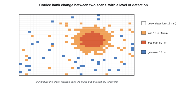
One epoch of the monitoring was flown with drone lidar when the crew could not reach the bank after heavy rain. Its uncertainty was larger, about 25 mm, and the level of detection for that comparison rose to about 50 mm, a reminder that combining different sensors in a monitoring series costs sensitivity unless their accuracy is matched.
Power line clearance
The power line that follows the canal for 6 km crosses the canal access road four times, and the district's maintenance trucks carry a crane. Clearance from conductors to the road, to the ground and to vegetation is checked from the classified mobile and airborne data. Each span's conductor points are fitted with a catenary curve, closely approximated over short spans by a parabola, and the lowest point and clearances are computed. The code fits a parabola through three conductor points over an 80 m span and finds the lowest point 7.75 m above the road surface.
A clearance measured on survey day is not the clearance on the worst day. Conductors sag more when hot, under heavy electrical load and under ice, and swing sideways in wind. Utilities therefore record the conductor temperature and line load at the time of survey and model the sag at maximum design temperature and ice load. The district does not own the line, so it sends the measured clearances, the survey time and the weather to the utility, which runs the analysis and confirms the safe operating limits for the crane. Vegetation encroachment, trees within a set distance of the conductors, is reported as a list of locations for the utility's vegetation management crews.
Canal cross-sections and condition
The mobile mapping survey gives a continuous model of the canal prism, from which Theo cuts cross-sections every 20 m and at every structure. Each section is compared with the design section from the 1950s drawings: flow area, wetted perimeter, bank heights and freeboard. Where sediment has built up or banks have slumped, the flow area is reduced and with it the canal's capacity. The section in the code, from a reach below the second coulee crossing, has lost 11 percent of its flow area to sediment on the bed and slumping of the lower banks. The canal was surveyed during the autumn drawdown, so the bed was exposed; where water remained, the green-laser data or a sonar run would be needed.
Seepage, the district's other concern, shows up indirectly: wet ground and lush vegetation along the outside of the banks, and settlement of the bank crest where water has carried fine material away. Comparing bank crest elevations with the design and with later surveys, and overlaying intensity and multispectral imagery that show wet ground, gives the district a ranked list of reaches for seepage investigation, which feeds the canal lining program.
Other uses of the corridor data
Once collected, a corridor lidar survey serves many users. The county's floodplain mapping uses the bare-earth model for hydraulic modeling of the river through the headworks. Forestry and agriculture use canopy height and crop structure: the shelterbelts along the canal are inventoried from the high vegetation class, and agronomists use slope and drainage from the bare earth for field drainage design. Planners use building and road classes. Archaeologists have found old trails and homestead foundations in shaded relief maps of the bare earth, features invisible in imagery. Because so many users benefit, the project's data are shared with the state, and through partnership with the 3D Elevation Program they become part of the national holdings available to everyone.
Sharing raises questions that are best settled in the contract: who owns the data, who may use and redistribute it, what metadata accompany it, and whether any parts are sensitive. Detailed scans of the headworks, for example, reveal the layout of control equipment, and the district decided to share the airborne data openly but keep the terrestrial scans of the gate house internal.
The project report
Leah assembled the final report. It begins with the purpose and the specifications, then describes each data set: equipment, dates, conditions, control, processing, registration or trajectory adjustment, classification and products. Accuracy is reported as lesson 10 describes, with checkpoint lists, swath statistics and registration residuals. Coordinate reference systems are stated completely, including realization, epoch, geoid model and projection, as GEOM-340 insisted. Limitations are explicit: areas with no ground returns, the deep pool surveyed by sonar, the elements of the headworks model taken from drawings, the drone epoch's lower accuracy. Metadata files accompany every data set in the formats the specifications require.
| Question | Decides |
|---|---|
| What decisions will the data support, and what accuracy and detail do they need? | System, density, accuracy class, LOD and LOA |
| What platform fits the area, the objects and the access? | Terrestrial, mobile, airborne, drone or bathymetric |
| What coordinate system, realization, epoch and height datum? | Control, geoid model, projection |
| What season, weather and site conditions are needed? | Leaf-off, snow-free, calm water, traffic closures |
| How will the data be checked? | Independent checkpoints, overlaps, swath and registration reports |
| What classes, products and formats are deliverable? | LAS or LAZ version, classes, bare earth, models, metadata |
| Who owns, shares and maintains the data? | Licenses, sensitivity, update responsibility |
| What are the safety hazards? | Laser class, traffic, water, heights, weather |
The checklist is a summary of this course. Each question was answered, sometimes the hard way, on the district's project: the berm lost by the ground filter, the ICP that converged to the wrong place on the canal reach, the algae bloom that would have wasted a bathymetric flight, the low-distortion projection that kept the headworks model at true scale. Lidar has made three-dimensional measurement cheap and fast; deciding what to measure, how well, and how to prove it remains the surveyor's and engineer's work.
Worked problem
Level of detection for a mixed-sensor comparison
A terrestrial epoch has an uncertainty of 6 mm, a drone lidar epoch 25 mm, and their registration 5 mm. What is the 95 percent level of detection, and can a 30 mm settlement of the crest be detected?
Show solution
- \[\text{LoD}_{95} = 1.96\sqrt{6^2 + 25^2 + 5^2} = 1.96\sqrt{36 + 625 + 25} = 1.96 \times 26.2 = 51\ \text{mm}\]
Answer: The level of detection is about 51 mm, so a 30 mm settlement cannot be distinguished from noise in this comparison; two terrestrial epochs (18 mm) would detect it.
Common mistakes
MistakeReporting a volume without its uncertainty.
InsteadState the base surface, the epochs' uncertainty and the resulting volume uncertainty.
MistakeTreating every cell beyond the level of detection as real change.
InsteadAbout 5 percent exceed a 95 percent threshold by chance; require spatial coherence.
MistakeReporting power line clearance on survey day as the design clearance.
InsteadRecord conditions; sag at maximum temperature and ice load must be modeled.
MistakeSharing all scans openly without considering sensitivity.
InsteadSettle ownership, licenses and sensitive content in the contract.
Summary and key terms
- Volumes compare a surface with a base; systematic errors dominate their uncertainty.
- Monitoring compares epochs registered on stable areas; the level of detection sets the smallest detectable change.
- Normal-based cloud comparison suits steep and complex surfaces better than vertical DEM differences.
- Power line clearances need conductor fitting and modeling of sag under design conditions.
- Cross-sections from mobile data quantify lost canal capacity and point to seepage problems.
- Corridor data serve many users; reports, metadata, sharing and safety complete the work.
- DEM of difference
- The grid of height differences between two surface models.
- Level of detection
- The smallest change distinguishable from noise at a stated confidence.
- M3C2
- A cloud-to-cloud comparison method measuring change along local normals with uncertainty.
- Catenary
- The curve of a hanging cable, approximated by a parabola over short spans.
- Clearance
- The distance between a conductor and the ground, a structure or vegetation.
- Flow area
- The cross-sectional area of water in a channel at a given level.
- Canopy height model
- The difference between a surface model and the bare earth, giving vegetation height.
Practice problems
Work each problem on paper first, then reveal the answer to check.
A 2 cm vertical offset affects two surveys of a 5 ha site. What volume error results?
Show answer
1,000 m³.
Each epoch has 10 mm uncertainty and registration 5 mm. What is the 95 percent level of detection?
Show answer
About 29 mm.
Why register monitoring epochs to bedrock and control pillars only?
Show answer
So real movement of the slope is not absorbed into the registration.
Why is a parabola acceptable for a short conductor span?
Show answer
It closely approximates the catenary when sag is small relative to span.
Name two users of corridor lidar other than the district.
Show answer
For example flood mapping and agriculture or forestry.
Lesson quiz · 5 questions
Score 60% or more to complete this lesson.
Create a free account to save your progress, take quizzes and earn a certificate.