Terrestrial laser scanners

The headworks gate structure is the project's most valuable and most fragile asset. Built in 1957, it has six concrete piers carrying a 64 m (210 ft) gate deck, radial gates between the piers, a gate house with hoists and pipework, and a fish ladder on the north bank. The concrete is spalling, one pier appears to lean, and the project's engineers want to design a rehabilitation from accurate as-built geometry rather than from the original drawings, which no longer match what was built. Ines chooses terrestrial laser scanning: a tripod-mounted scanner can record every surface of the structure to a few millimeters in a few days, without anyone climbing onto the gates.

How a terrestrial scanner works

A terrestrial laser scanner combines a rangefinder (lesson 1) with two angle measurements. A mirror, usually rotating continuously, sweeps the beam in a vertical plane, while the whole upper part of the instrument turns slowly about the vertical axis. Encoders read both angles for every pulse. The scanner therefore measures, for each point, a range \(R\), a horizontal angle \(\alpha\) and a vertical angle \(\beta\), which it converts to Cartesian coordinates in its own frame:

Most modern scanners cover a full dome, 360° horizontally and about 270° to 300° vertically, leaving only a cone below the tripod unseen. Panoramic scanners of this kind are the workhorses of building, plant and heritage work. Camera-type scanners with a narrower field of view, and long-range scanners designed for mines, open pits and landslides at ranges of a kilometer or more, fill other niches. A dual-axis compensator in most instruments measures the tilt of the vertical axis so that the scan can be leveled, which helps registration and allows the scanner to be set up over a known point like a total station.

Scanners differ in their ranging method (pulsed, phase or hybrid), range, measurement rate, noise and angular accuracy. Typical figures for a current mid-range panoramic scanner are a measurement rate of up to a million points per second, a usable range of 0.5 m to a few hundred meters, range noise of 1 to 2 mm at 10 m on a gray surface, and angular accuracy of about 5 to 10 arcseconds. Specifications are measured under ideal conditions on cooperative targets, so Ines reads them as a ceiling rather than as the performance the crew will achieve on wet concrete at 40 m.

Resolution, spacing and quality settings

The scanner's operator chooses an angular step, often expressed as a point spacing at a reference range such as 6.3 mm at 10 m. The spacing on a surface is the step multiplied by the range, divided by the cosine of the incidence angle if the surface is oblique:

Halving the step quadruples the number of points and roughly quadruples the scan time. Operators also choose a quality or averaging setting, which fires several pulses per point and averages them to reduce noise, again at the cost of time. A rule Ines teaches new staff: choose the spacing from the smallest feature that must be modeled, not from what the scanner can do. Modeling a 25 mm bolt head needs spacing of a few millimeters; modeling the outline of a pier needs perhaps 10 mm. Over-dense scans waste field time and storage and slow every later step.

Spacing is not resolution. The footprint of the beam (lesson 1) limits how small a feature can be distinguished: if the footprint is larger than the spacing, adjacent points overlap and fine detail is smeared. Some manufacturers quote an effective resolution that combines both.

import math
# Scanner settings on the headworks survey
step_mrad = 0.31        # angular step between points (one of the scanner's presets)
range_noise = 0.0012    # 1-sigma range noise at 10 m on a mid-reflectance target, m
pulse_rate = 500000     # points per second

def spacing(R, step=step_mrad):
    return R * step / 1000.0

print("range  spacing  spacing on a surface at 60 deg incidence")
for R in (5, 10, 20, 40, 80):
    s = spacing(R)
    print(f"{R:4d} m {s*1000:7.1f} mm {s/math.cos(math.radians(60))*1000:9.1f} mm")

# Full-dome scan time
cols = 2 * math.pi / (step_mrad / 1000)
rows = math.pi * 0.85 / (step_mrad / 1000)   # about 85 percent of the half circle in elevation
n = cols * rows
print(f"\npoints per full scan {n/1e6:.1f} million, time {n/pulse_rate/60:.1f} min")

# How many setups for the gate deck: maximum range set by the required spacing
need = 0.006                                     # 6 mm spacing on the concrete
Rmax = need / (step_mrad / 1000) * math.cos(math.radians(45))
print(f"range for 6 mm spacing at 45 deg incidence: {Rmax:.1f} m")
deck = 64.0                                      # gate deck length, m
print(f"setups along the 64 m deck (both sides, 30 % overlap): {2*math.ceil(deck/(2*Rmax*0.7))}")

# Range noise grows with range and with darker, steeper surfaces (simple model)
def sigma(R, rho=0.4, inc=0.0):
    return range_noise * math.sqrt((R / 10) ** 2 * (0.4 / rho) / max(math.cos(math.radians(inc)), 0.05))
for R, rho, inc in ((10, 0.4, 0), (30, 0.4, 0), (30, 0.1, 0), (30, 0.4, 70)):
    print(f"R {R:2d} m rho {rho:.1f} inc {inc:2d}: sigma {sigma(R, rho, inc)*1000:.1f} mm")

range  spacing  spacing on a surface at 60 deg incidence
   5 m     1.6 mm       3.1 mm
  10 m     3.1 mm       6.2 mm
  20 m     6.2 mm      12.4 mm
  40 m    12.4 mm      24.8 mm
  80 m    24.8 mm      49.6 mm

points per full scan 174.6 million, time 5.8 min
range for 6 mm spacing at 45 deg incidence: 13.7 m
setups along the 64 m deck (both sides, 30 % overlap): 8
R 10 m rho 0.4 inc  0: sigma 1.2 mm
R 30 m rho 0.4 inc  0: sigma 3.6 mm
R 30 m rho 0.1 inc  0: sigma 7.2 mm
R 30 m rho 0.4 inc 70: sigma 6.2 mm

With the chosen step of 0.31 mrad the scanner delivers 3.1 mm spacing at 10 m but 12.4 mm at 40 m, and twice that on surfaces met at 60°. A full dome at this setting is about 175 million points and takes about six minutes at 500,000 points per second; in practice the crew restricts the field of view to the structure. To hold 6 mm on surfaces seen at up to 45°, ranges must stay below about 14 m, which gives four setups along each side of the deck, eight in all, before the gate house, the piers' faces and the fish ladder are counted. The noise model shows the other cost of range: noise triples from 10 m to 30 m and doubles again on a dark or steeply inclined surface.

Planning a scan project

A scan plan answers four questions: what surfaces must be captured, at what spacing and accuracy, from where, and how the setups will be tied together. Ines works from a site visit and the old drawings, marking every surface the engineers need: the upstream and downstream faces of each pier, the gate deck top and soffit, the gate arms and trunnions, the gate house interior and the fish ladder walls. She then places setups so that each surface is seen at reasonable range and incidence from at least one, and preferably two, positions, because a second view fills shadows and provides redundancy.

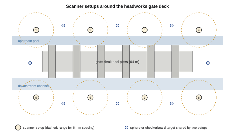
Shadows, called occlusions, are the main enemy. Every object hides what lies behind it, so the piers hide each other's faces, the handrail hides the deck edge, and the gate arms hide the trunnions. Setups on the deck itself, on the banks and on a boat in the upstream pool were all considered; the district agreed to lower the pool for two days so that the crew could scan the upstream pier faces from the dry apron. Inside the gate house, where pipes and hoists crowd a small room, setups are closer together, sometimes every 3 or 4 m.

Ties between setups are planned at the same time (lesson 5). With target-based registration, each pair of neighboring setups must see at least three common targets, well spread in three dimensions and preferably more, so that a single disturbed target can be detected. With cloud-to-cloud registration, neighboring scans need generous overlap, perhaps 30 percent, on surfaces with varied geometry. On this project Ines uses both: sphere targets and black-and-white checkerboards for the main chain of setups, and cloud-to-cloud matching to add the gate house setups.

Control and georeferencing

Scans are first measured in each scanner's own frame. To place the structure in project coordinates, and to tie it to the airborne and mobile data collected later, some targets are surveyed by total station or GNSS from control. Grant's crew runs a closed traverse from two district control monuments on either bank and measures each control target by two sets of angles and distances. The scanner can also be set up over a known point and oriented to a backsight like a total station, a method called traverse scanning, which some instruments support with a built-in compensator and a sighting device.

Coordinates for the headworks are in NAD83(2011) with orthometric heights in NAVD 88, projected on the project's low-distortion projection designed in GEOM-340 so that grid distances match ground distances within a few parts per million. That choice matters for scanning: a scan is measured at true ground scale, and placing it on a projection with a scale factor of 0.9993 would shrink the 64 m deck by 45 mm.

Field procedure

A typical setup takes ten to twenty minutes. The operator sets up and levels the tripod, checks that targets are visible, enters the project, setup name and settings, starts the scan, and while it runs records notes and photographs. Many scanners capture panoramic images with an internal camera after the scan, for adding color to the points; these images take extra time and need consistent light, so the crew schedules interior and exterior work to avoid harsh sun. Field checks before leaving each setup include reviewing the scan on the tablet for gaps, confirming that every planned target was captured, and checking the preliminary registration that many systems compute on site.

Conditions affect the result. Strong sunlight raises background noise for some scanners; rain and fog scatter the beam and produce noise points; vibration from traffic or running machinery disturbs the instrument; wind shakes the tripod and the vegetation. At the headworks the river's roar is harmless, but the trucks crossing the deck shake it noticeably, so the crew scans the deck during an agreed traffic closure. Cold weather shortens battery life and can fog optics when the instrument is carried from a warm truck.

Errors and calibration of terrestrial scanners

Like a total station, a scanner has instrumental errors: the axes are not perfectly perpendicular, the laser is not perfectly aligned with the mirror, the range has a small constant offset and scale error, and the vertical angle index is not exactly zero. Manufacturers calibrate these in the factory and recommend periodic recalibration, typically yearly. Many instruments also offer a field check that scans targets from two faces or compares distances with known values. Lesson 10 returns to calibration; for now the practical point is that a scanner with an expired calibration certificate or a recent knock should be checked against known distances before an important project.

Surface properties add errors no calibration can remove. Shiny metal, such as the stainless guides beside the gates, can reflect the beam away or produce false points by multiple reflection; very dark surfaces produce noisy, sometimes biased ranges; and translucent materials let the beam enter before reflecting, so that ranges to snow, ice, marble or some plastics come out slightly long. Edges produce mixed pixels. Wet concrete, common at a headworks, is darker than dry concrete and noisier.