Network analysis

Two of the questions in Leah's needs assessment could not be answered with overlay or straight-line distance. The maintenance foreman wanted to know the quickest way from the district yard to a damaged culvert, on roads that ranged from paved highway to a canal service road that was passable only in dry weather. The water manager wanted to know, when a check structure on the main canal was closed for repair, which turnouts would lose water and how much ordered flow would be cut off. Both are questions about networks: sets of connected lines along which things move. The first is a transportation network, where crews travel in either direction; the second is a flow network, where water moves only downstream. This lesson covers how networks are modeled, the shortest path algorithm at the heart of most network analysis, the standard network problems, and the tracing operations used for utilities such as canals, pipes and power lines.

Networks as graphs

A network is modeled as a graph: a set of nodes (junctions, also called vertices) connected by edges (links). In a road network, nodes are intersections and road ends, and edges are road segments between them. In the canal network, nodes are structures and junctions, and edges are the reaches between them. Each edge has an impedance, the cost of traversing it: length, travel time, fuel, or for a canal a hydraulic property. Edges may be undirected, traversable either way, or directed, traversable only in one direction, such as a one-way street or a canal reach. Turns at nodes may carry their own costs or be prohibited, such as a left turn across a divided highway or a U-turn on a narrow service road. Edges may also carry restrictions that apply to some users only, such as a weight limit on a bridge that stops the district's excavator truck but not a pickup.

Building a network dataset from line features requires topology (Lesson 2). Lines must meet at shared nodes where connections exist, and must not be connected where they only cross, as at an overpass. Software usually connects lines at shared end points and, optionally, at shared vertices, and uses elevation fields or connectivity rules to keep crossing roads apart. A road layer drawn as spaghetti with gaps of a few centimeters at intersections produces a network in which most destinations cannot be reached at all, and the first test of any network is to check that every node can be reached from a central point.

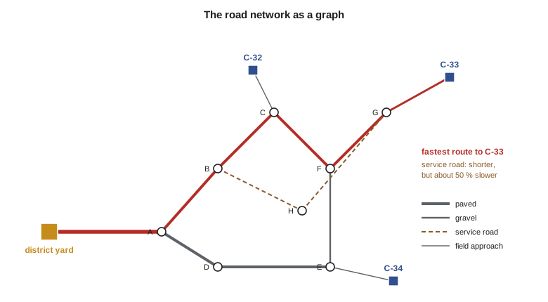
Leah built the road network from the county road data and the Census Bureau's TIGER/Line roads, adding the district's canal service roads, which appear in no public dataset, from the GNSS survey. Each edge was given a speed by road class: 50 mph on paved highways, 35 mph on gravel county roads, 15 mph on canal service roads and 20 mph on field approaches to structures. Seasonal restrictions closed the service roads when the district's road condition flag was set after rain.

Shortest paths

The shortest path problem asks for the route of least total impedance between two nodes. Edsger Dijkstra's algorithm, published in 1959, solves it for non-negative impedances. It keeps a tentative cost for every node, starting at zero for the origin and infinity elsewhere, and a set of nodes whose cost is final. At each step it takes the unfinished node with the smallest tentative cost, marks it final, and relaxes its edges: for each neighbor, if the cost through the current node is lower than the neighbor's tentative cost, it lowers that cost and records the current node as the neighbor's predecessor. When the destination is final, following predecessors back from it gives the path. With a priority queue the algorithm runs in time roughly proportional to the number of edges times the logarithm of the number of nodes, fast enough for networks of millions of edges.

Dijkstra's algorithm explores outward in all directions. The A* algorithm adds a heuristic estimate of the remaining cost to the destination, such as the straight-line distance divided by the highest speed, and explores nodes in order of cost so far plus estimated cost to go, reaching the destination after exploring far fewer nodes. Because the estimate never exceeds the true remaining cost, A* still finds the optimal path. Routing services on the web use further techniques that preprocess the network so that queries across a continent take milliseconds.

import heapq
# Road network: node -> list of (adjacent node, length mi, speed mph). Gravel range roads are slower; the canal
# service road is one-way-safe only in dry weather, so it is given a low speed.
edges = [("yard", "A", 2.0, 50), ("A", "B", 1.0, 35), ("B", "C", 1.0, 35), ("A", "D", 1.0, 50), ("D", "E", 2.0, 50),
         ("C", "F", 1.0, 35), ("E", "F", 1.0, 35), ("F", "G", 1.0, 35), ("B", "H", 1.5, 15), ("H", "G", 1.2, 15),
         ("C", "C-32", 0.25, 20), ("G", "C-33", 0.4, 20), ("E", "C-34", 0.55, 20)]
graph = {}
for a, b, km, v in edges:
    t = km / v * 60                                   # minutes (km holds miles here)
    graph.setdefault(a, []).append((b, t, km)); graph.setdefault(b, []).append((a, t, km))
def dijkstra(src):
    best, prev, pq = {src: 0.0}, {}, [(0.0, src)]
    while pq:
        t, u = heapq.heappop(pq)
        if t > best[u]: continue
        for v, w, _ in graph[u]:
            if t + w < best.get(v, 1e9):
                best[v] = t + w; prev[v] = u; heapq.heappush(pq, (t + w, v))
    return best, prev
best, prev = dijkstra("yard")
def path(v):
    p = [v]
    while p[-1] in prev: p.append(prev[p[-1]])
    return p[::-1]
for c in ("C-32", "C-33", "C-34"):
    p = path(c); km = sum(next(k for n, _, k in graph[a] if n == b) for a, b in zip(p, p[1:]))
    print(f"yard -> {c}: {best[c]:5.1f} min, {km:.1f} mi via {' - '.join(p)}")
print("service area within 7 minutes of the yard:", sorted(n for n, t in best.items() if t <= 7))

# Canal network: each reach flows from an upstream node to a downstream node (a directed tree)
reaches = {"headworks": ["check 1"], "check 1": ["check 2", "L5"], "check 2": ["check 3"], "check 3": ["check 4", "L7"],
           "check 4": ["check 5", "L8"], "check 5": ["reservoir"], "L5": [], "L7": [], "L8": []}
turnouts = {"L5": 14, "L7": 23, "L8": 17, "check 4": 3, "check 5": 2, "reservoir": 0}   # turnouts on each reach
orders = {"L5": 39.0, "L7": 83.0, "L8": 57.0, "check 4": 6.4, "check 5": 4.2}         # ordered flow, cfs
def downstream(node):
    out, stack = [], list(reaches[node])
    while stack:
        n = stack.pop(); out.append(n); stack.extend(reaches.get(n, []))
    return out
cut = ["check 4"] + downstream("check 4")      # the reach below check 4 and everything downstream
print(f"\nclosing check 4 cuts off: {sorted(cut)}")
print(f"turnouts affected: {sum(turnouts.get(n, 0) for n in cut)}, ordered flow lost {sum(orders.get(n, 0) for n in cut):.1f} cfs")
up = [n for n in reaches if "check 4" in downstream(n)]
print("upstream structures that could be used to hold water back:", up)

yard -> C-32:   6.6 min, 4.2 mi via yard - A - B - C - C-32
yard -> C-33:  10.5 min, 6.4 mi via yard - A - B - C - F - G - C-33
yard -> C-34:   7.7 min, 5.5 mi via yard - A - D - E - C-34
service area within 7 minutes of the yard: ['A', 'B', 'C', 'C-32', 'D', 'E', 'yard']

closing check 4 cuts off: ['L8', 'check 4', 'check 5', 'reservoir']
turnouts affected: 22, ordered flow lost 67.6 cfs
upstream structures that could be used to hold water back: ['headworks', 'check 1', 'check 2', 'check 3']

The fastest route to culvert C-33 takes 10.5 minutes over 6.4 miles of highway and gravel road. The route along the canal service road is shorter, about 6.1 miles, but at 15 mph it takes about 16 minutes, so the algorithm avoids it. Minimizing time and minimizing distance give different answers whenever speeds differ, and the impedance must match the question: time for dispatch, distance for fuel or mileage claims. Within 7 minutes of the yard, the crew can reach six road nodes and culvert C-32, which is the service area used to decide which structures the yard crew covers and which the crew based at the north end of the district covers.

Standard network problems

Most network analysis in practice uses a few standard problems built on shortest paths. A closest facility analysis finds, for each incident, the nearest facility by network cost, such as the closest of two crew bases to a washout, or the nearest structures to a reported spill. A service area analysis finds all parts of the network within a cost of a facility, such as everything within 15 minutes of the yard, and is drawn as a set of edges or a polygon around them. An origin-destination cost matrix gives the network cost between every origin and every destination and is the input to many planning models. Location-allocation chooses the best sites for facilities among candidates, such as where to put a second equipment yard to minimize average response time to structures. Vehicle routing designs routes for several vehicles visiting many stops with time windows and capacities, such as the ditch riders' daily rounds of turnouts, and generalizes the traveling salesperson problem, which asks for the shortest tour visiting every stop once. These routing problems cannot be solved exactly for large numbers of stops in reasonable time, so software uses heuristics that find good but not necessarily optimal routes.

The ditch riders' rounds showed the value of these tools. Each rider visited 30 to 50 turnouts a day to set gates and read meters. Routing their visits with the actual orders for the day, rather than following the same fixed order along each lateral, shortened the average round by about a fifth in the first season, mostly by avoiding backtracking along laterals with no orders.

Flow networks and tracing

Utility networks, such as canals, water mains, sewers, gas pipelines and electrical distribution, differ from road networks in that the commodity moves according to the network's physical state, not the choice of a traveler. A canal network is a directed graph: water flows from the headworks through the main canal and checks to laterals and turnouts. Its basic analyses are traces. A downstream trace from a point finds every element that receives water through that point; an upstream trace finds every element that supplies it. An isolation trace finds the valves or gates that must be closed to isolate a section for repair. Traces follow connectivity and the status of devices: a closed gate stops a trace, and an open bypass continues it.

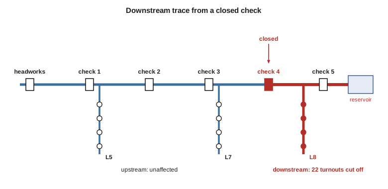
In the code, closing check 4 cuts off the reach below it, Lateral 8, check 5 and the reservoir, with 22 turnouts and the flow ordered for them. An upstream trace lists the structures that can hold water back while the repair is done. In practice the water manager used the trace to produce the list of affected water users from the turnouts through the fields and ownership tables, and to decide whether orders below check 4 could be served from the reservoir by reversing a pump, which the network's device rules represented as a conditional connection.

Utility network models used by large utilities go further. They classify features into devices, lines and junctions with rules about which may connect to which, keep subnetworks such as pressure zones or circuits, and support hydraulic or electrical models that compute flows and pressures. The district's needs were met by a simpler geometric network with directed edges and device status, which Theo kept in the database and validated after each edit: every turnout had to be reachable downstream from the headworks, and no reach could flow uphill according to its recorded inverts.