Cartography and map design

Most people would meet the district's GIS through maps: the wall map in the board room, the map printed with each landowner's annual statement, the seepage-risk map in the engineer's report and the screens on the ditch riders' tablets. A map that is accurate but hard to read fails as surely as one that is wrong. The first draft of the board's water use map, produced quickly from the software's defaults, used a rainbow of colors for seven classes of water use, a legend with values to four decimal places and the district boundary in the same weight as the roads; the chair asked which color meant 'a lot'. This lesson covers the principles that make maps work: purpose and audience, visual hierarchy and the visual variables, classification of quantitative data, color, typography, generalization and the ethics of map making.

Purpose, audience and medium

Every map starts from three questions: what is it for, who will read it, and how will they read it? The board's water use map was for comparing fields at a glance in a meeting, read by non-specialists from a few meters away, on paper. The ditch riders' tablet map was for finding turnouts and reading orders in a truck, read at arm's length in bright sun, on a small screen with touch. The engineer's seepage map was for analysis and a permanent record, read closely by specialists, and had to state its methods and uncertainty. These purposes lead to different choices of extent, scale, content, symbols and detail, and a single 'GIS map' that tries to serve all of them serves none well.

Thematic maps show the distribution of one or a few variables, such as water use or seepage risk; reference maps show the locations of many kinds of features, such as roads, laterals and structures, for finding one's way. Thematic maps should keep the base information to the minimum needed to locate the theme, drawn quietly in gray, so that the theme stands out.

Map elements and layout

A finished map usually has a title that says what and where, the map body, a legend explaining every symbol not obvious from context, a scale bar (a graphic bar remains correct when the map is enlarged or reduced, unlike a stated ratio), a north arrow where north is not obviously up, and a source and credit statement with the date and the coordinate reference system. Insets and locator maps show where the area lies within a larger region. Layout arranges these elements so that the map body dominates and the eye moves naturally from title to map to legend; the elements are aligned to a grid and given space to breathe rather than crowded into corners.

Visual hierarchy and visual variables

Visual hierarchy is the ordering of map content so that the most important information is seen first. It is created by contrast: in size, lightness, color saturation and line weight. On the water use map, the field shading is the figure and everything else is ground; the district boundary is a medium dark line, roads are thin gray lines, and labels for townships are small and light. A common mistake is to draw every layer at full strength, so that roads, boundaries and the theme compete equally for attention.

Jacques Bertin's visual variables describe the ways a symbol can vary: position, size, shape, lightness (value), hue, saturation, orientation and texture. They differ in what they can show. Size and lightness are ordered, so they suit quantitative and ordinal data: bigger or darker reads as more. Hue and shape are not ordered, so they suit nominal categories: crop types, structure types. Using hue for a quantity, as the rainbow scheme did, forces the reader to consult the legend for every field and invites misreading, because the eye does not see red as 'more' than blue. Quantities that are totals, such as the volume delivered to each turnout, are best shown by proportional symbols sized by the value; rates and densities, such as water use per hectare, by shading areas (a choropleth map). Shading areas by totals misleads, because large fields look important simply for being large.

Classifying quantitative data

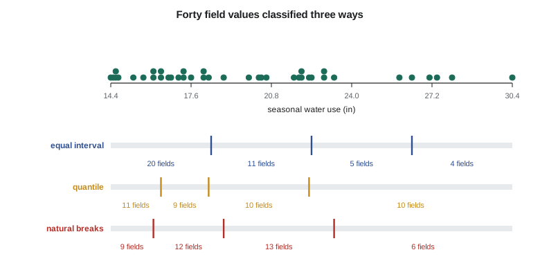
Choropleth maps usually group values into a few classes, each shown by one shade, because readers can distinguish only about five to seven lightness steps reliably. How the class breaks are chosen changes the map's message. Equal interval classes divide the range into equal widths, which is easy to read but can leave most fields in one class when the data are skewed. Quantile classes put equal numbers of features in each class, which uses all shades but can split nearly equal values and lump very different ones. Natural breaks (the Jenks method) place breaks where the data have gaps, by minimizing the variance within classes; the goodness of variance fit (GVF), one minus the ratio of within-class to total squared deviations, measures how well the classes describe the data. Standard deviation classes show departure from the mean and suit diverging data. Breaks can also be chosen manually at meaningful values, such as the district's allocation per hectare, which is often best for a decision-making audience.

import math
# Seasonal crop water use of 40 fields on Lateral 7 (inches), from the remote sensing program
v = [14.4, 14.5, 14.6, 14.6, 14.7, 15.3, 15.7, 16.1, 16.1, 16.4, 16.4, 16.7, 16.8, 17.1, 17.3, 17.3, 17.6, 18.1, 18.1, 18.3,
     18.9, 19.9, 20.3, 20.4, 20.6, 21.7, 21.9, 22.0, 22.0, 22.3, 22.4, 22.9, 22.9, 23.3, 25.9, 26.4, 27.1, 27.4, 28.0, 30.4]
UNIT = "in"
k = 4
def classes(breaks): return [sum(1 for x in v if lo < x <= hi or (i == 0 and x == lo)) for i, (lo, hi) in enumerate(zip(breaks, breaks[1:]))]
def gvf(breaks):            # goodness of variance fit: 1 - (within-class deviations / total deviations)
    m = sum(v) / len(v); sdam = sum((x - m) ** 2 for x in v); sdcm = 0.0
    for i, (lo, hi) in enumerate(zip(breaks, breaks[1:])):
        c = [x for x in v if lo < x <= hi or (i == 0 and x == lo)]
        cm = sum(c) / len(c); sdcm += sum((x - cm) ** 2 for x in c)
    return 1 - sdcm / sdam
lo, hi = min(v), max(v)
eq = [lo + (hi - lo) * i / k for i in range(k + 1)]
qu = [v[0]] + [v[round(len(v) * i / k) - 1] for i in range(1, k)] + [v[-1]]
# Fisher-Jenks natural breaks by dynamic programming (optimal for sorted data)
n = len(v); INF = float("inf")
def ssd(i, j):              # sum of squared deviations of v[i:j]
    c = v[i:j]; m = sum(c) / len(c); return sum((x - m) ** 2 for x in c)
cost = [[INF] * (n + 1) for _ in range(k + 1)]; cut = [[0] * (n + 1) for _ in range(k + 1)]
cost[0][0] = 0.0
for c in range(1, k + 1):
    for j in range(c, n + 1):
        for i in range(c - 1, j):
            t = cost[c - 1][i] + ssd(i, j)
            if t < cost[c][j]: cost[c][j], cut[c][j] = t, i
idx, j = [], n
for c in range(k, 0, -1): idx.append(j); j = cut[c][j]
idx = sorted(idx)
jb = [v[0]] + [v[i - 1] for i in idx]
for name, b in (("equal interval", eq), ("quantile", qu), ("natural breaks", jb)):
    print(f"{name:15s} breaks " + ", ".join(f"{x:.1f}" for x in b) + f" {UNIT}; counts {classes(b)}; GVF {gvf(b):.3f}")

# Douglas-Peucker simplification of the Lateral 7 line for small-scale maps
line = [(0, 0), (40, 6), (95, 4), (150, 22), (210, 31), (260, 28), (330, 60), (390, 95), (430, 101), (480, 140),
        (540, 162), (600, 160), (655, 190), (700, 240), (760, 262), (820, 266), (880, 300), (930, 345), (1000, 352)]
def perp(p, a, b):
    if a == b: return math.dist(p, a)
    return abs((b[0] - a[0]) * (a[1] - p[1]) - (a[0] - p[0]) * (b[1] - a[1])) / math.dist(a, b)
def dp(pts, tol):
    if len(pts) < 3: return pts
    d, i = max((perp(p, pts[0], pts[-1]), i) for i, p in enumerate(pts[1:-1], 1))
    if d <= tol: return [pts[0], pts[-1]]
    return dp(pts[:i + 1], tol)[:-1] + dp(pts[i:], tol)
for tol in (2, 10, 25):
    s = dp(line, tol)
    print(f"tolerance {tol:2d} m: {len(s):2d} of {len(line)} vertices kept")

equal interval  breaks 14.4, 18.4, 22.4, 26.4, 30.4 in; counts [20, 11, 5, 4]; GVF 0.910
quantile        breaks 14.4, 16.4, 18.3, 22.3, 30.4 in; counts [11, 9, 10, 10]; GVF 0.879
natural breaks  breaks 14.4, 16.1, 18.9, 23.3, 30.4 in; counts [9, 12, 13, 6]; GVF 0.946
tolerance  2 m: 19 of 19 vertices kept
tolerance 10 m: 12 of 19 vertices kept
tolerance 25 m:  3 of 19 vertices kept

The water use values are skewed: most fields used 14 to 23 inches, and six alfalfa fields used more than 25 inches. Equal intervals put half the fields in the lowest class and only four in the top class. Quantiles should give ten fields per class, but two fields with exactly 16.4 inches fall on a break, so the classes hold 11 and 9; quantile breaks also lump fields of 22.4 and 30.4 inches together. Natural breaks find the gaps near 16.1, 18.9 and 23.3 inches and fit the data best, with a GVF of 0.946. For the board, Leah used natural breaks rounded to 16, 19 and 24 inches, so that the legend read in round numbers and the top class matched the alfalfa fields the board was asking about.

Color

Color schemes should match the data. Sequential schemes, light to dark in one or two hues, suit data that run from low to high, such as water use. Diverging schemes, two hues meeting at a light neutral midpoint, suit data with a meaningful middle, such as change since last year or departure from the allocation. Qualitative schemes, distinct hues of similar lightness, suit categories such as crop types. The ColorBrewer schemes, developed by Cynthia Brewer for cartographers, are widely available in GIS software and were designed with these rules. Rainbow schemes have no consistent order of lightness, create false boundaries where hues change abruptly and are hard to read for people with color vision deficiency.

Roughly one man in twelve and one woman in two hundred has some form of color vision deficiency, most commonly difficulty distinguishing red from green. Maps that rely on red against green, such as good against bad condition, lose that information for many readers. Using lightness as well as hue, testing schemes with a deficiency simulator and adding labels or patterns for critical distinctions avoid the problem. The district's condition map for culverts used a sequential scheme from light yellow to dark red with distinct symbol shapes for the worst class, so that it read correctly in grayscale photocopies as well.

Typography and labeling

Labels identify features and carry much of a map's information. Type should be legible at the reading distance, with a limited set of fonts, usually one family in several weights and sizes. Type style signals feature class: water features are often in italic blue, settlements in upright black, and size follows importance. Placement follows conventions that readers expect: point labels above and to the right of the symbol where space allows; line labels along the line, following its curve, above it; area labels spread across the area. Labels should not overlap each other or important symbols, and automatic placement engines in GIS software do much of this work, but critical labels often need manual adjustment. Halos, thin outlines around text in the background color, keep labels legible over busy imagery.

Generalization

As scale decreases, maps must show less. Cartographic generalization includes selection (omitting less important features, such as field approaches on the district map), simplification (removing detail from lines and boundaries), smoothing, aggregation (merging small fields into blocks), displacement (moving features apart that would otherwise overlap, such as a road and the lateral beside it) and exaggeration (widening a lateral so it remains visible). The Douglas-Peucker algorithm, published in 1973, simplifies lines by keeping the vertex farthest from the line joining the ends if it lies beyond a tolerance, and repeating on each half; vertices within the tolerance are dropped. In the code, a tolerance of 10 m keeps 12 of 19 vertices of a lateral segment and 25 m keeps only 3, suitable for a district overview at 1:100,000, where 25 m is a quarter of a millimeter. Simplification of shared boundaries must be done topologically, so that neighboring polygons stay joined.

Maps for screens

Screen maps differ from paper. They are viewed at many scales, so content and symbols should change with zoom level: the ditch riders' map showed only laterals and structures below 1:50,000 and added turnout numbers, field boundaries and orders as they zoomed in. Screens are smaller, so legends are often hidden in panels and replaced by pop-ups that show a feature's attributes on a tap. Bright sun washes out subtle colors, so the tablet map used stronger contrasts than the board's paper map. Web maps also need to meet accessibility requirements (Lesson 12), which affect color contrast and the availability of the same information without the map.

Ethics and honesty

Every map is a selection, and selections can mislead. Class breaks can make a problem look large or small; a color scheme can make a modest change look alarming; omitting the uncertainty of an interpolated surface makes it look like measurement. Maps of personal information, such as each landowner's water use, can expose private information even when no names appear, because readers can identify fields. Leah's rule for the district was that every published map should state its source, date and method, show the data on which interpolated surfaces rest, use classes that the board had agreed in advance, and never show individual water use to anyone other than the user and authorized staff.