Raster data models

Not everything the district needed to know came in neat features. The elevation model, the soil capability map, the crop map and water use estimates from the remote sensing program, the orthophotos and the depth to groundwater were all quantities that vary from place to place, and the remote sensing products already arrived as grids of pixels. Leah wanted a seepage risk map for the reaches where the canal ran on embankment, which meant combining several of these layers cell by cell. That is the domain of the raster data model. This lesson describes how rasters are organized and stored, how they are tied to coordinates, and the families of operations, called map algebra, that turn input rasters into new ones.

Cells, resolution and extent

A raster divides space into a regular grid of cells, usually square, arranged in rows and columns. Each cell holds one value for each band: an elevation, a soil class, a reflectance, a count. The cell size is the raster's spatial resolution, the length of a cell side on the ground. The extent is the area the grid covers, given by the coordinates of its edges, and the number of rows and columns follows from the extent and cell size. A raster of the 30,000 ha service area at 1 m resolution has about 300 million cells; at 30 m it has about 330,000. Halving the cell size quadruples the number of cells, so resolution is always a trade between detail and the volume of data and processing.

A cell value represents the whole cell, but what it represents depends on how the value was produced. It may be the value at the cell center (an elevation sampled from a surface), an average over the cell (a reflectance measured by a sensor), the dominant class (a land cover map), or a total (the number of wells in the cell). The difference matters when rasters are combined or resampled: averaging a set of dominant-class values produces nonsense, and summing average values double counts.

Rasters also differ in what their values mean. Continuous rasters, such as elevation, temperature or water use, hold measurements on interval or ratio scales. Categorical (thematic) rasters, such as soil class, land cover or crop type, hold codes for classes on a nominal or ordinal scale, with a table that gives the meaning of each code. Cells for which no value exists, outside the surveyed area or under cloud, are flagged with a special NoData value, and every operation must decide how to treat them. A NoData value of zero is dangerous where zero is also a valid value, such as a depth or a slope on flat ground.

Tying a raster to coordinates

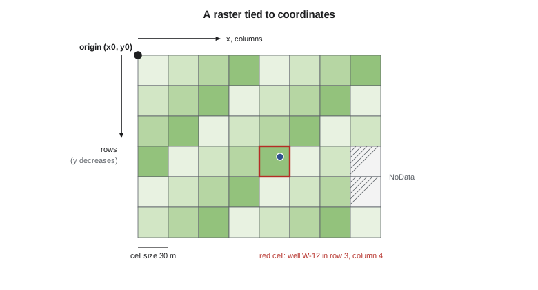
A raster is georeferenced by an affine transformation, often called the geotransform, that converts row and column numbers into map coordinates. For a north-up raster it needs only the coordinates of the upper-left corner, \(x_0\) and \(y_0\), and the cell size \(c\). The coordinates of the center of the cell in row \(r\) and column \(k\), both counted from zero, are

and the cell containing a point follows by inverting these relations and rounding down. Note that rows increase downward while northing increases upward, which is why the second equation has a minus sign; mixing the conventions is a classic cause of rasters that appear upside down. The general affine form adds rotation terms for rasters that are not aligned with the grid, and the parameters are stored in the file header or in a small companion text file called a world file. Rasters are always in some coordinate reference system, and reprojecting a raster means computing, for each output cell, where it falls in the input and resampling there.

Data types, bands and storage

Cell values are stored with a fixed data type, which sets the range and precision available and the file size. An 8-bit unsigned integer holds 0 to 255 and suits class codes and many image bands; 16-bit integers suit most satellite reflectance data scaled by a factor; 32-bit floating point suits elevations and model outputs. Storing a class map as 32-bit floats wastes four times the space; storing elevations as 8-bit integers loses everything below a meter or above 255 m. A raster may have several bands with the same grid, such as the red, green, blue and near-infrared bands of an orthophoto, or the twelve monthly values of a climate variable.

Raster files are large, so they are compressed. Lossless methods, such as run-length encoding, LZW and DEFLATE, reproduce values exactly and work especially well on categorical rasters with long runs of equal values. Lossy methods, such as JPEG, discard detail the eye barely notices and are suitable for imagery used as a backdrop, never for data that will be analyzed. Large rasters are also divided into tiles, square blocks read independently, and store overviews, reduced-resolution copies used when the whole raster is displayed at small scale. GeoTIFF is the most widely used format, and the cloud-optimized GeoTIFF arranges tiles and overviews so that a program can read just the part it needs over the internet, which is how many public elevation and imagery archives are now served. Multidimensional data, such as daily weather grids, are often stored in NetCDF or Zarr.

Choosing between raster and vector

Neither model is better in general. Rasters represent continuous fields naturally, make overlay of many layers simple and fast because cells line up, and match the form of imagery and elevation data. They represent boundaries only to the nearest cell, so a 30 m raster cannot say whether a 24 m wide canal lies on one side of a fence or the other, and their size grows with the square of resolution. Vectors represent discrete features precisely and compactly, carry rich attributes and topology, and support network analysis, but overlay of many polygon layers is computationally heavy and produces many small slivers. Most real projects use both, converting between them as needed. Converting vectors to rasters (rasterization) assigns each cell the value of the feature covering its center or most of its area; converting rasters to vectors (vectorization) traces the boundaries of zones of equal value, producing stair-stepped edges unless they are smoothed.

Map algebra

Map algebra, formalized by C. Dana Tomlin in the 1980s, treats rasters as variables in expressions and groups operations by which cells contribute to each output cell. Local operations compute each output cell from the input cells at the same location only: adding two rasters, reclassifying soil codes, applying a condition such as 'soil class at most 3 and slope under 5 %'. Focal operations compute each output cell from a neighborhood around it, such as a 3 × 3 window: a moving average, a maximum, a slope calculation (Lesson 9) or an edge filter. Zonal operations compute statistics for zones defined by another raster, such as the mean slope within each field, and either report them in a table or write them back to every cell of the zone. Global operations use the whole raster, such as the distance from every cell to the nearest canal cell or the cost of traveling from each cell to a road.

Reclassification is the most common local operation. Soil survey codes, crop codes or slope values are mapped to new classes or scores through a lookup table, often as the first step of a suitability or risk analysis. Overlays then combine the reclassified rasters by logical conditions (Boolean overlay) or weighted sums (weighted overlay). Boolean overlay is easy to explain but treats a slope of 4.9 % and 0.5 % alike and a slope of 5.1 % as entirely unsuitable. Weighted overlay assigns scores and weights; it is more flexible but its result depends on the scores and weights chosen, which should be agreed with the people who will use it and tested for sensitivity.

# A small raster: 6 rows x 8 columns of 30 m cells, upper-left corner at (2400.0, 3180.0) in the district grid
x0, y0, cell = 2400.0, 3180.0, 30.0
def to_cell(x, y):  return int((y0 - y) // cell), int((x - x0) // cell)          # (row, col)
def to_xy(r, c):    return x0 + (c + 0.5) * cell, y0 - (r + 0.5) * cell          # middle of the cell
print("well W-12 at (2547.0, 3061.0) falls in cell", to_cell(2547.0, 3061.0))
print("middle of cell (2, 5) is at", to_xy(2, 5))

# Soil capability class (1 best ... 5 poor) and slope in per cent, one value per cell; -9 is NoData
soil = [[2, 2, 2, 3, 3, 4, 4, 5],
        [2, 2, 2, 3, 3, 4, 4, 5],
        [1, 1, 2, 2, 3, 3, 4, 4],
        [1, 1, 1, 2, 2, 3, 3, -9],
        [1, 1, 1, 2, 2, 2, 3, -9],
        [1, 1, 1, 1, 2, 2, 2, 3]]
slope = [[1.0, 1.2, 1.5, 2.0, 2.8, 4.1, 6.5, 9.0],
         [0.8, 1.0, 1.3, 1.8, 2.5, 3.9, 6.0, 8.2],
         [0.6, 0.7, 1.0, 1.4, 2.2, 3.0, 4.8, 7.1],
         [0.5, 0.6, 0.8, 1.1, 1.9, 2.6, 4.0, -9],
         [0.4, 0.5, 0.7, 0.9, 1.5, 2.1, 3.2, -9],
         [0.4, 0.4, 0.6, 0.8, 1.2, 1.8, 2.7, 3.5]]
ND = -9
# Local operation: suitable for sprinkler irrigation if soil class <= 3 and slope < 5 %
suit = [[ND if s == ND or g == ND else int(s <= 3 and g < 5.0) for s, g in zip(rs, rg)] for rs, rg in zip(soil, slope)]
print("\nsuitability (1 = suitable, 0 = not, -9 = NoData)")
for row in suit: print(" ".join(f"{v:2d}" for v in row))
n1 = sum(v == 1 for row in suit for v in row)
print(f"suitable area {n1} cells x {cell * cell:.0f} m2 = {n1 * cell * cell / 10000:.2f} ha")

# Focal operation: 3 x 3 mean of slope, ignoring NoData and the edge
def focal_mean(g, r, c):
    v = [g[i][j] for i in range(r - 1, r + 2) for j in range(c - 1, c + 2)
         if 0 <= i < len(g) and 0 <= j < len(g[0]) and g[i][j] != ND]
    return sum(v) / len(v)
print(f"\nfocal mean slope at (1, 6): {focal_mean(slope, 1, 6):.2f} %; at (3, 6): {focal_mean(slope, 3, 6):.2f} %")

# Zonal operation: mean slope in each field zone
zones = [[1, 1, 1, 1, 2, 2, 2, 2]] * 3 + [[3, 3, 3, 3, 2, 2, 2, 2]] * 3
for z in (1, 2, 3):
    v = [slope[r][c] for r in range(6) for c in range(8) if zones[r][c] == z and slope[r][c] != ND]
    print(f"field zone {z}: {len(v)} cells, mean slope {sum(v) / len(v):.2f} %, max {max(v):.1f} %")

# Run-length encoding of the first row of the soil raster
def rle(row):
    out, cur, n = [], row[0], 0
    for v in row:
        if v == cur: n += 1
        else: out.append((cur, n)); cur, n = v, 1
    return out + [(cur, n)]
print("\nrun-length encoding of soil row 0:", rle(soil[0]))

well W-12 at (2547.0, 3061.0) falls in cell (3, 4)
middle of cell (2, 5) is at (2565.0, 3105.0)

suitability (1 = suitable, 0 = not, -9 = NoData)
 1  1  1  1  1  0  0  0
 1  1  1  1  1  0  0  0
 1  1  1  1  1  1  0  0
 1  1  1  1  1  1  1 -9
 1  1  1  1  1  1  1 -9
 1  1  1  1  1  1  1  1
suitable area 38 cells x 900 m2 = 3.42 ha

focal mean slope at (1, 6): 5.84 %; at (3, 6): 3.83 %
field zone 1: 12 cells, mean slope 1.19 %, max 2.0 %
field zone 2: 22 cells, mean slope 3.85 %, max 9.0 %
field zone 3: 12 cells, mean slope 0.64 %, max 1.1 %

run-length encoding of soil row 0: [(2, 3), (3, 2), (4, 2), (5, 1)]

In the example, 38 of the 48 cells meet both conditions, covering 3.42 ha, and the two NoData cells stay NoData rather than being counted as unsuitable. The focal mean of slope at row 1, column 6 is 5.84 % because the window reaches into the steeper cells to the east, while the same cell's own value is 6.0 %. Focal operations near the raster edge use fewer neighbors, and the code averages only those that exist; other choices, such as padding the edge with copies of the outermost cells, give slightly different results. Zone 2, on the coulee side of the field, has a mean slope of 3.85 % but a maximum of 9.0 %, which shows why zonal statistics are reported with more than the mean.

Resampling

Whenever a raster is reprojected, aligned to another grid or changed in resolution, the values of the new cells must be estimated from the old ones. Nearest-neighbor resampling takes the value of the closest input cell; it preserves the original values and must be used for categorical rasters, but it produces blocky results and positional shifts of up to half a cell. Bilinear interpolation takes a distance-weighted average of the four nearest cells and cubic convolution uses sixteen; both produce smoother results for continuous data such as elevation, but they create new values that did not exist in the input and blur sharp edges. When a raster is coarsened, aggregation by mean, majority, minimum or maximum is often more appropriate than resampling, and the choice should follow from what the cell value means.

The district's soil information came from the Natural Resources Conservation Service's soil survey as polygons with tabular properties, which Theo rasterized at 10 m to match the Sentinel-2 crop map, using the map unit covering each cell center. The elevation model came from the 3D Elevation Program's 1 m lidar-derived model, which he aggregated to 10 m by the mean for the seepage study and kept at 1 m for terrain work near structures. Every derived raster was snapped to the same 10 m grid in the State Plane system, so that cells lined up exactly and no resampling was needed for overlay.