
GEOM-330 · Lesson 2 of 12 · 23 min
Vector data models
The first layers the district needed were vector layers: the canal and its laterals, the structures on them, the turnouts that deliver water to fields, the fields themselves and the parcels of land they lie on. Theo's first job was to inspect what already existed. The CAD drawing of the main canal had the centerline on one layer and the banks on another, drawn as hundreds of short line segments that did not always meet. The ditch riders' turnout lists gave a lateral and a number, such as 7-14, but no coordinates. The field boundaries from the remote sensing project were polygons digitized on orthophotos, and the parcel boundaries came from the public parcel layer. Before converting anything, Leah and Theo had to decide how each kind of feature would be modeled. This lesson covers the vector data model: the geometry types, how they are stored, how topology records the relationships between them, and how attributes and linear referencing attach information to them.
Points, lines and polygons
The vector model represents features by coordinates. A point is a single coordinate pair (or triple, with height): a turnout, a well, a culvert, a gauge. A line, more precisely a polyline or line string, is an ordered sequence of points joined by straight segments: a canal centerline, a road, a pipeline. A polygon is an area bounded by a closed ring, a line string whose first and last points coincide: a field, a parcel, a reservoir. Polygons may have holes (inner rings), such as a farmyard excluded from a field, and a feature may have several parts, such as a parcel split by a road, stored as a multipart geometry. Curves such as circular arcs are approximated by many short segments in most systems, although some formats store true arcs, which matters for legal boundaries and road alignments.
Whether a feature is a point, a line or a polygon depends on the scale and the purpose. A turnout is a point on a district map and a small concrete structure with a gate, a measuring weir and a pipe on a construction drawing. The canal is a line for network analysis and a polygon of water surface for a seepage study. The district modeled the canal as a centerline network, with the right-of-way as a separate polygon layer, because the main questions were about connectivity and distances along the canal.
Each coordinate also needs a precision. Storing coordinates to a millimeter is harmless for surveyed turnouts, but storing digitized field boundaries to a millimeter suggests an accuracy they do not have. Spatial databases also apply a tolerance when comparing coordinates, the distance within which two points are treated as the same, and choosing a tolerance much larger than the data accuracy merges features that should be separate.
Simple features and storage
The Simple Features standard of the Open Geospatial Consortium (OGC), also published as ISO 19125, defines the geometry types used by nearly all modern GIS software and spatial databases: Point, LineString, Polygon, their multi versions and GeometryCollection, with optional Z (height) and M (measure) values. It also defines rules for valid geometry. A valid polygon's rings must close, must not cross themselves, and its holes must lie inside the outer ring and must not overlap one another. Invalid polygons, such as a field boundary that loops back over itself, cause analysis tools to give wrong areas or fail entirely, so validity checks are part of every data load. Geometries are exchanged as well-known text (WKT), a readable form such as POLYGON((0 0, 805 0, 805 610, 590 802, 0 802, 0 0)), or as well-known binary for efficiency.
Simple features are stored in many file formats. The shapefile, introduced in the early 1990s, is still common but has serious limits: each dataset is several files that must travel together, attribute names are limited to ten characters, files are limited to 2 GB, there is no proper support for null values or long text, and the coordinate reference system is in a separate file that is often lost. GeoPackage, an OGC standard, stores many layers, their CRS definitions, rasters and even styles in one SQLite database file and has become the preferred open format for exchange. GeoJSON, a text format standardized by the Internet Engineering Task Force, is the common format for web applications; its current specification requires longitude and latitude on WGS 84, so data must be transformed before export. Spatial databases (Lesson 4) store geometry as a column type alongside ordinary attributes.
Spaghetti and topology
In the simplest vector model, each feature is stored independently as its own list of coordinates, without any record of how it relates to other features. This is called the spaghetti model, and it is what CAD drawings and many shapefiles provide. Two neighboring fields that share a boundary each store that boundary separately. If one copy is edited and the other is not, the result is a sliver gap or overlap between them. Two lines that look connected on screen may in fact stop a few centimeters short of each other, which is invisible on a map but fatal to network analysis, because the software sees no connection.
Topology records the spatial relationships between features explicitly: which lines meet at which nodes, which polygons lie on each side of a boundary, which polygons are adjacent. In the classic arc-node model, lines (arcs) begin and end at nodes; each arc stores its from-node and to-node and the polygons on its left and right; and each polygon is defined by the arcs that bound it. A shared boundary is stored once, so neighboring polygons cannot develop gaps or overlaps, and connectivity can be followed directly from the stored relationships. Modern systems usually store simple features and enforce topology through rules checked during editing: lines must not have dangles, polygons must not overlap, turnouts must lie on a lateral, fields must lie within the district boundary.
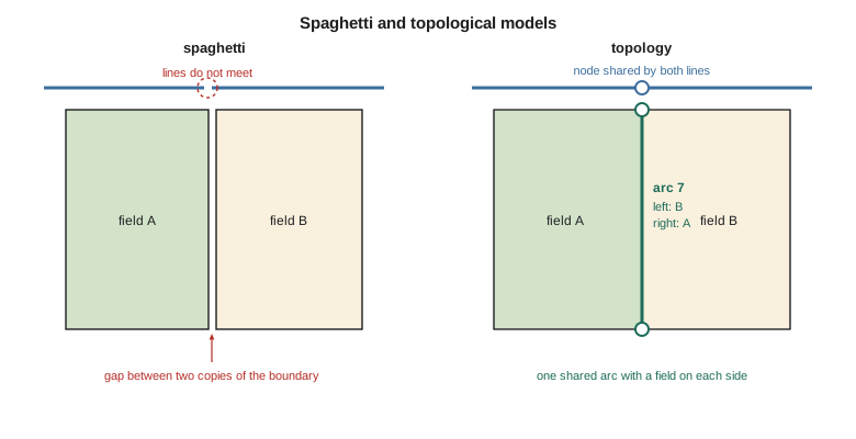
The three properties that topology captures are connectivity (which lines join), adjacency (which areas touch) and containment (which features lie inside which areas). They are properties that survive stretching and bending of a map, which is why the word comes from the branch of mathematics that studies such properties. A district map drawn badly out of scale would still show that turnout 7-14 lies on Lateral 7 and inside field 7-14, and that is exactly the information the network trace and the water order system need.
Attributes and keys
Each feature has attributes stored in a table, one row per feature and one column per attribute. Attributes have types: integers, real numbers, text, dates, Booleans. They are also measured on different scales, which limits what can be done with them. Nominal attributes are names or categories, such as crop type or structure type; they can be counted but not ordered. Ordinal attributes have an order but not meaningful differences, such as a condition rating from 1 (failed) to 5 (good). Interval attributes have meaningful differences but no true zero, such as temperature in degrees Celsius or a year. Ratio attributes have a true zero, so ratios are meaningful: water delivered, field area, pipe diameter. Averaging condition ratings or dividing years produces numbers that look meaningful and are not.
Every feature needs a stable identifier that does not change when its geometry or attributes change and is never reused. The ditch riders' turnout numbers, such as 7-14, were meaningful to staff but not stable: when a turnout was added between 7-14 and 7-15, it had been called 7-14A, and when Lateral 7 was extended, some turnouts were renumbered. Theo gave every feature a system identifier and kept the ditch riders' number as an ordinary attribute, so that a renumbering would never break links to water orders and inspections. Domains restrict attributes to valid values, so that structure type can only be one of gate, check, drop, culvert, weir or siphon, and the condition rating only an integer from 1 to 5.
| Layer | Geometry | Key attributes | Topology rules |
|---|---|---|---|
| Canal network | Line, with measures | Lateral name, capacity, lining, year built | No dangles except at ends; connected to the main canal |
| Structures | Point | Type, size, material, year installed, condition | Must lie on the canal network |
| Turnouts | Point | Ditch rider number, pipe size, measuring device | Must lie on a lateral; must be served by one field |
| Fields | Polygon | Field number, irrigated area, irrigation method | No overlaps; within the district boundary |
| Parcels | Polygon (public data) | Legal description, title reference | Not edited by the district |
| Right-of-way | Polygon | Width, acquisition plan | Contains the canal centerline |
Computing with vector geometry
Many GIS calculations come down to simple geometry on coordinate lists. The area of a polygon follows from the shoelace formula, which sums cross products of successive vertices:
with the last vertex joined back to the first. The sign of the sum gives the ring's orientation: positive for counter-clockwise, negative for clockwise. Conventions differ (the shapefile stores outer rings clockwise, the GeoJSON specification asks for counter-clockwise), so software checks orientation when reading. The centroid of a polygon is computed from similar sums. Point-in-polygon testing is usually done by ray casting: draw a ray from the point in one direction and count how many times it crosses the boundary; an odd count means inside. Distances from a point to a line are computed segment by segment, projecting the point onto each segment and keeping the nearest.
import math
# Field 7-14 in district grid coordinates (easting, northing in m); the lateral cuts the north-east corner
field = [(0, 0), (805, 0), (805, 610), (590, 802), (0, 802)]
def area_perimeter_centroid(poly):
    a = cx = cy = p = 0.0
    n = len(poly)
    for i in range(n):
        x1, y1 = poly[i]; x2, y2 = poly[(i + 1) % n]
        cross = x1 * y2 - x2 * y1
        a += cross; cx += (x1 + x2) * cross; cy += (y1 + y2) * cross
        p += math.hypot(x2 - x1, y2 - y1)
    a /= 2
    return abs(a), p, (cx / (6 * a), cy / (6 * a)), "counter-clockwise" if a > 0 else "clockwise"
A, P, (gx, gy), order = area_perimeter_centroid(field)
print(f"area {A:,.0f} m2 = {A / 10000:.2f} ha, perimeter {P:,.1f} m, centroid ({gx:.1f}, {gy:.1f}), ring {order}")

def inside(pt, poly):            # ray casting: count crossings of a ray to the east
    x, y = pt; c = False
    for i in range(len(poly)):
        (x1, y1), (x2, y2) = poly[i], poly[i - 1]
        if (y1 > y) != (y2 > y) and x < x1 + (y - y1) * (x2 - x1) / (y2 - y1):
            c = not c
    return c
for name, pt in (("turnout 7-14", (742, 655)), ("turnout 7-15", (770, 760))):
    print(f"{name} at {pt}: {'inside' if inside(pt, field) else 'outside'} field 7-14")

# Linear referencing along Lateral 7 (vertices of the lateral line, chainage measured from the main canal)
lat7 = [(-400, 1200), (300, 1060), (590, 802), (805, 610), (1400, 330)]
cum = [0.0]
for (x1, y1), (x2, y2) in zip(lat7, lat7[1:]):
    cum.append(cum[-1] + math.hypot(x2 - x1, y2 - y1))
print(f"\nLateral 7 length {cum[-1]:,.1f} m")
def locate(m):                   # coordinates at chainage m
    for i in range(len(lat7) - 1):
        if cum[i] <= m <= cum[i + 1]:
            t = (m - cum[i]) / (cum[i + 1] - cum[i])
            (x1, y1), (x2, y2) = lat7[i], lat7[i + 1]
            return x1 + t * (x2 - x1), y1 + t * (y2 - y1)
def measure(pt):                 # chainage and offset of the nearest point on the line
    best = None
    for i in range(len(lat7) - 1):
        (x1, y1), (x2, y2) = lat7[i], lat7[i + 1]
        dx, dy = x2 - x1, y2 - y1
        t = max(0.0, min(1.0, ((pt[0] - x1) * dx + (pt[1] - y1) * dy) / (dx * dx + dy * dy)))
        qx, qy = x1 + t * dx, y1 + t * dy
        d = math.hypot(pt[0] - qx, pt[1] - qy)
        side = "left" if dx * (pt[1] - y1) - dy * (pt[0] - x1) > 0 else "right"
        if best is None or d < best[1]:
            best = (cum[i] + t * math.hypot(dx, dy), d, side)
    return best
m, off, side = measure((742, 655))
km = int(m // 1000)
print(f"turnout 7-14 is at chainage {km}+{m - 1000 * km:05.1f}, offset {off:.1f} m {side}")
x, y = locate(1500.0)
print(f"chainage 1+500 is at ({x:.1f}, {y:.1f})")area 624,970 m2 = 62.50 ha, perimeter 3,095.3 m, centroid (391.6, 389.9), ring counter-clockwise turnout 7-14 at (742, 655): inside field 7-14 turnout 7-15 at (770, 760): outside field 7-14 Lateral 7 length 2,047.9 m turnout 7-14 is at chainage 1+313.3, offset 8.4 m right chainage 1+500 is at (904.3, 563.3)
The field covers 62.50 ha, and turnout 7-14 lies inside it, while the point recorded for 7-15 lies just outside, on the far side of the lateral's corner, which is where the ditch rider said it was. The centroid falls near the middle of the field, but for an L-shaped or crescent-shaped polygon the centroid can fall outside the polygon, which matters when centroids are used to place labels or to join features to the polygons containing them. Many systems therefore offer a 'point on surface' guaranteed to lie inside.
Linear referencing
People who work along linear features locate things by distance along them, not by coordinates. Highway crews use kilometer posts, pipeline operators use stationing, and the district's ditch riders described every structure by its chainage, the distance in meters from the start of the lateral, written in the form 1+313 for 1,313 m. A linear referencing system stores routes as lines with measures (the M values of simple features) and locates events along them by measure. Point events, such as a turnout at 1+313, need one measure; linear events, such as a lined reach from 0+400 to 1+150, need two. Events are stored in an ordinary table and placed on the map dynamically by dynamic segmentation, so that a reach can be added or changed without editing the line geometry.
Measures do not have to equal the geometric length. The district's chainages had been measured along the as-built centerline in the 1950s, and in places the realigned canal was a few meters shorter or longer than the old one. Theo calibrated the measures to surveyed chainage markers at structures, so that a ditch rider's chainage and the GIS chainage agreed, and recorded the calibration points so that later realignments could be handled the same way.
Worked problem
Chainage and offset of a turnout
Turnout 7-14 was surveyed at (742, 655) in the district grid. Lateral 7 runs through (590, 802) and (805, 610), and the chainage at (590, 802) is 1,102.1 m. Find the turnout's chainage and its offset from the centerline.
Show solution
- \[\mathbf{d} = (805 - 590,\ 610 - 802) = (215,\ -192), \quad |\mathbf{d}| = 288.3 \text{ m}\]
- \[t = \frac{(742 - 590)(215) + (655 - 802)(-192)}{288.3^2} = \frac{32\,680 + 28\,224}{83\,089} = 0.733\]
- \[m = 1102.1 + 0.733 \times 288.3 = 1313.4 \text{ m}\]
- The offset is the distance from the turnout to the foot of the perpendicular, here about 8 m.
Answer: The turnout is at chainage 1+313, matching the code\'s 1+313.3 to rounding, with an offset of 8.4 m to the right of the direction of flow. Chainages should always be computed from the stored, calibrated geometry rather than scaled from a drawing.
Three dimensions and time
Vector features may carry heights as Z values: the invert elevations of culverts, the crest elevation along an embankment, the top of a well casing. A network of pipes or channels with inverts can then be checked for slope, a quick test of whether water can flow where the drawings say it does. Time is usually stored as attributes, such as an installation date and a removal date, so that a layer can show the system as it was in any year. The district kept removed structures in the same layer with a removal date instead of deleting them, so that questions about the past, such as when a culvert was last replaced, could still be answered.
Common mistakes
MistakeConverting CAD lines straight into a network layer.
InsteadClean and snap the lines so that they meet at nodes, then validate the topology.
MistakeUsing meaningful numbers such as 7-14 as the only key.
InsteadGive every feature a stable system identifier; keep local numbers as attributes.
MistakeExporting GeoJSON in projected coordinates.
InsteadTransform to longitude and latitude on WGS 84 for standard GeoJSON.
MistakeAveraging an ordinal condition rating.
InsteadReport the distribution or the median of ordinal attributes.
MistakeStoring shapefiles without their .prj file.
InsteadKeep the CRS with the data; prefer GeoPackage, which stores it internally.
Summary and key terms
- Vector data represent features by coordinates as points, lines and polygons, possibly multipart, with optional heights and measures.
- The OGC Simple Features standard defines the geometry types and validity rules used by most systems.
- GeoPackage and spatial databases avoid most shapefile limitations; GeoJSON uses WGS 84 longitude and latitude.
- Topology records connectivity, adjacency and containment; spaghetti data must be cleaned before network or overlay analysis.
- Attributes have types and measurement scales that limit which operations are meaningful.
- Stable identifiers and domains protect the integrity of a database over time.
- Linear referencing locates events by measure along routes, matching how staff describe locations along canals and roads.
- Polyline
- An ordered sequence of points joined by straight segments.
- Simple Features
- The OGC and ISO standard for vector geometry types and their validity rules.
- Topology
- The explicit relationships of connectivity, adjacency and containment between features.
- Dangle
- A line end that does not connect to another line where it should.
- Domain
- The set of valid values for an attribute.
- Linear referencing
- Locating features by measure along a linear route.
- Dynamic segmentation
- Placing events stored in a table onto routes by their measures.
- Well-known text
- A text encoding of vector geometry defined by the Simple Features standard.
Practice problems
Work each problem on paper first, then reveal the answer to check.
Find the area of the triangle (0, 0), (300, 0), (0, 200).
Show answer
½ |300 × 200| = 30,000 m² = 3.0 ha.
A ray from a point crosses a polygon boundary three times. Is the point inside?
Show answer
Yes; an odd number of crossings means inside.
Why is a shared field boundary stored once in a topological model?
Show answer
So neighboring polygons cannot develop gaps or overlaps when edited.
Is a culvert's year of installation nominal, ordinal, interval or ratio?
Show answer
Interval: differences are meaningful but year zero is not a true zero.
A lined reach runs from 0+400 to 1+150. How long is it?
Show answer
750 m.
Lesson quiz · 5 questions
Score 60% or more to complete this lesson.
Create a free account to save your progress, take quizzes and earn a certificate.